金樓子卷四‧梁‧孝元皇帝
見善則喜,聞惡則憂,民之情也。茍無憂喜,其惟聖人乎?若無喜而不喜,無憂而不憂,蓋何足稱也。白鳥,蚊也。齊桓公臥於栢寢 ,謂仲父曰︰吾國富民殷,無餘憂矣。一物失所,寡人猶為之悒悒 ,今白鳥營營,饑而未飽,寡人憂之。因開翠紗之幬,進蚊子焉。其蚊有知禮者,不食公之肉而退。其蚊有知足者●公而退。其蚊有不知足者,遂長噓短吸而食之;及其飽也,腹膓為之破潰。公曰︰嗟乎民生亦猶是。乃宣下齊國脩止足之鑒,節民玉食,節民錦衣,齊國大化。
以蚊子立論,能得國之大化??當真匪夷所思,不知何處想來!!既已為白鳥立傳,打不得也。事實白鳥有複眼,反應要比人快的多 ,想打怕也打不到的哩!!??觀物聯想以至於如此者,大概上能閱覽天文卦象,下可讀通地理風水的吧??!!
因此以近攝鏡之理,通廣角鏡頭
Wide-angle lens
In photography and cinematography, a wide-angle lens refers to a lens whose focal length is substantially smaller than the focal length of a normal lens for a given film plane. This type of lens allows more of the scene to be included in the photograph, which is useful in architectural, interior and landscape photography where the photographer may not be able to move farther from the scene to photograph it.
Another use is where the photographer wishes to emphasise the difference in size or distance between objects in the foreground and the background; nearby objects appear very large and objects at a moderate distance appear small and far away.
This exaggeration of relative size can be used to make foreground objects more prominent and striking, while capturing expansive backgrounds.[1]
A wide angle lens is also one that projects a substantially larger image circle than would be typical for a standard design lens of the same focal length. This large image circle enables either large tilt & shift movements with a view camera, or a wide field of view.
By convention, in still photography, the normal lens for a particular format has a focal length approximately equal to the length of the diagonal of the image frame or digital photosensor. In cinematography, a lens of roughly twice the diagonal is considered “normal”.[2]
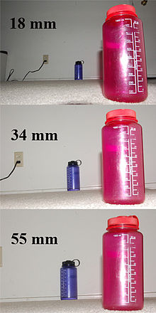
How focal length affects photograph composition. Three images depict the same two objects, kept in the same positions. By changing focal length and adjusting the camera’s distance from the pink bottle, it remains the same size in the image, while the blue bottle’s size appears to dramatically change. Also note that at small focal lengths, more of the scene is included.
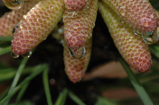
以及魚眼鏡頭
Fisheye lens
A fisheye lens is an ultra wide-angle lens that produces strong visual distortion intended to create a wide panoramic or hemispherical image.[1][2] Fisheye lenses achieve extremely wide angles of view by forgoing producing images with straight lines of perspective (rectilinear images), opting instead for a special mapping (for example: equisolid angle), which gives images a characteristic convex non-rectilinear appearance.
The term fisheye was coined in 1906 by American physicist and inventor Robert W. Wood based on how a fish would see an ultrawide hemispherical view from beneath the water (a phenomenon known as Snell’s window).[2][3] Their first practical use was in the 1920s for use in meteorology[4][5] to study cloud formation giving them the name “whole-sky lenses”. The angle of view of a fisheye lens is usually between 100 and 180 degrees[1] while the focal lengths depend on the film format they are designed for.
Mass-produced fisheye lenses for photography first appeared in the early 1960s[6] and are generally used for their unique, distorted appearance. For the popular 35 mm film format, typical focal lengths of fisheye lenses are between 8 mm and 10 mm for circular images, and 15–16 mm for full-frame images. For digital cameras using smaller electronic imagers such as 1/4″ and 1/3″ format CCD or CMOS sensors, the focal length of “miniature” fisheye lenses can be as short as 1 to 2mm.
These types of lenses also have other applications such as re-projecting images filmed through a fisheye lens, or created via computer generated graphics, onto hemispherical screens. Fisheye lenses are also used for scientific photography such as recording of aurora and meteors, and to study plant canopy geometry and to calculate near-ground solar radiation. They are also used as peephole door viewers to give the user a wide field of view.
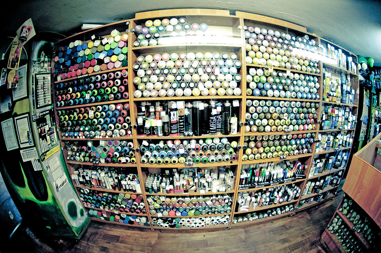
An example of full-frame fisheye used in a closed space (Nikkor 10.5mm)
之用,誠餘論矣。雖然。因為 CPU、GPU 之便宜與快速,影像處理軟體突飛猛進,或將賦予事物以新意乎☆★
Chessboard detection
Chessboards arise frequently in computer vision theory and practice because their highly structured geometry is well-suited for algorithmic detection and processing. The appearance of chessboards in computer vision can be divided into two main areas: camera calibration and feature extraction. This article provides a unified discussion of the role that chessboards play in the canonical methods from these two areas, including references to the seminal literature, examples, and pointers to software implementations.
……
Multiplane calibration
Multiplane calibration is a variant of camera auto-calibration that allows one to compute the parameters of a camera from two or more views of a planar surface. The seminal work in multiplane calibration is due to Zhang.[4] Zhang’s method calibrates cameras by solving a particular homogeneous linear system that captures the homographic relationships between multiple perspective views of the same plane. This multiview approach is popular because, in practice, it is more natural to capture multiple views of a single planar surface – like a chessboard – than to construct a precise 3D calibration rig, as required by DLT calibration. The following figures demonstrate a practical application of multiplane camera calibration from multiple views of a chessboard.[5]
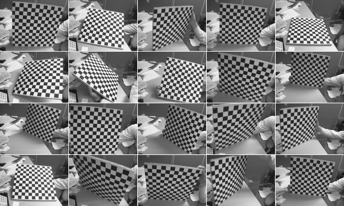
Multiple views of a chessboard for multiplane calibration
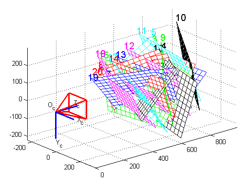
Reconstructed orientations (camera-centric coordinates)
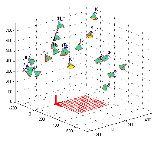
Reconstructed orientations (world-centric coordinates)
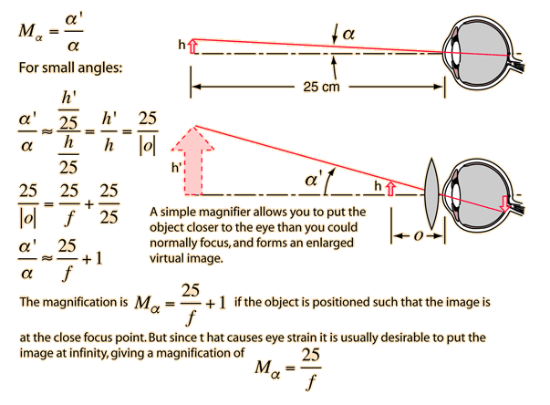
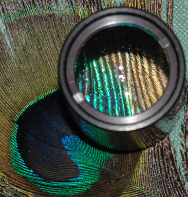
 公分。因此在觀察小東西時。需要放大鏡才能看的更清楚物件之紋理。若將放大鏡緊貼眼睛,就彷彿相機加裝

 。從
。從  ,解之得
,解之得
 。
。 ,
,


 越靠近焦點
越靠近焦點  ,虛像將趨近於與物同邊之無窮遠處
  。若以接續成像來講,此時眼睛與放大鏡中間的距離,對比下大可以忽略不計。因此從相對角放大率觀之,

 1:
1:


 、
、  之正負號時並不方便。何不以前焦點面
  、後焦點面
、後焦點面  將之改寫為
將之改寫為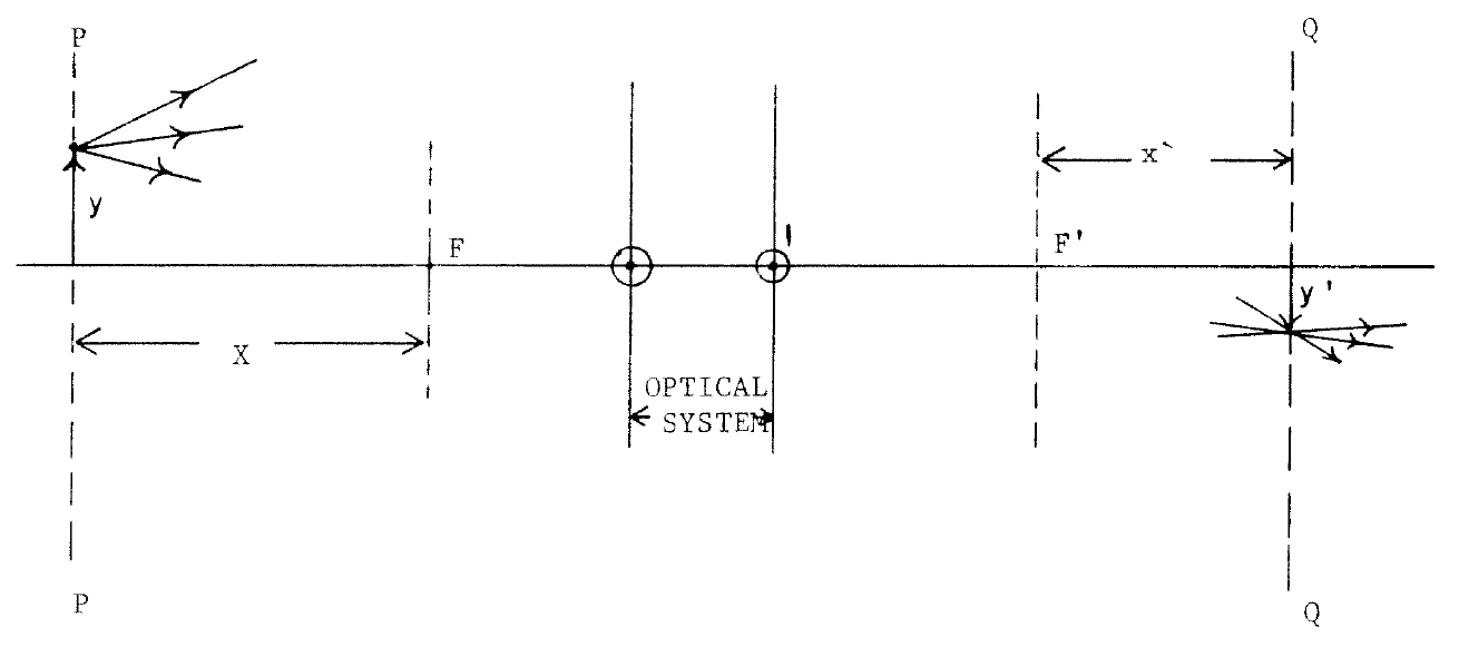
 。
。 。
。
 在前焦距
在前焦距  之前為正,在前焦距之後為負;
  在後焦距
在後焦距  之後為正,後焦距之前為負。故而方便以焦距
  為尺,探討物、像之位置也。


 ,得
,得  ;以及
;以及  ,得
,得  。誠有好處的也。
 。
。
 Click image for more views


 的所有整數解。
 的
的 ,其中的
,其中的 稱為勾股數。例如
 就是一組勾股數組。
 ,其中
,其中 。
。
 的整數解。
的整數解。 ,而後行經此光學系統 ,最終發生折射處【※ 或反射】稱之為『後端點』
  。這構成了『端點面參考系』,也就是『前後焦距』以平行光『度量』聚散的座標系。簡單推導如下︰
![ipython3 Python 3.4.2 (default, Oct 19 2014, 13:31:11) Type "copyright", "credits" or "license" for more information. IPython 2.3.0 -- An enhanced Interactive Python. ? -> Introduction and overview of IPython's features. %quickref -> Quick reference. help -> Python's own help system. object? -> Details about 'object', use 'object??' for extra details. In [1]: from sympy import * In [2]: from sympy.physics.optics import FreeSpace, FlatRefraction, ThinLens, GeometricRay, CurvedRefraction, RayTransferMatrix In [3]: init_printing() In [4]: A, B, C, D = symbols('A, B, C, D') In [5]: 光學系統 = RayTransferMatrix(A, B, C, D) In [6]: 光學系統 Out[6]: ⎡A B⎤ ⎢ ⎥ ⎣C D⎦ In [7]: z, h, θ = symbols('z, h, θ') In [8]: 平行光匯聚於後焦點 = FreeSpace(z) * 光學系統 * GeometricRay(h, 0) In [9]: 平行光匯聚於後焦點 Out[9]: ⎡h⋅(A + C⋅z)⎤ ⎢ ⎥ ⎣ C⋅h ⎦ In [10]: 匯聚前焦點之光而後平行 = 光學系統 * FreeSpace(z) * GeometricRay(0, θ) In [11]: 匯聚前焦點之光而後平行 Out[11]: ⎡θ⋅(A⋅z + B)⎤ ⎢ ⎥ ⎣θ⋅(C⋅z + D)⎦ In [12]: </pre> <span style="color: #003300;">得到</span> <span style="color: #003300;">後焦距 =](http://www.freesandal.org/wp-content/ql-cache/quicklatex.com-5390d7c4ed005cbe6eb166fa0a7341e0_l3.png "Rendered by QuickLaTeX.com") -\frac{A}{C}
-\frac{A}{C} -\frac{D}{C}
 \frac{1 - A}{C}
 \frac{1 - D}{C}
![</span> 故可驗證薄透鏡之等效式為︰ <pre class="lang:python decode:true">In [12]: 等效薄透鏡 = FreeSpace((1-A)/C) * 光學系統 * FreeSpace((1-D)/C) In [13]: 等效薄透鏡 Out[13]: ⎡ D⋅(-A + 1) -D + 1⎤ ⎢1 B + ────────── + ──────⎥ ⎢ C C ⎥ ⎢ ⎥ ⎣C 1 ⎦ In [14]: 等效薄透鏡.B.simplify() Out[14]: -A⋅D + B⋅C + 1 ────────────── C In [15]: </pre> <span style="color: #003300;"> 若此光學系統處於同一介質中,則</span>](http://www.freesandal.org/wp-content/ql-cache/quicklatex.com-7438f5f6242acbbf450b6f0fdcf22ba9_l3.png "Rendered by QuickLaTeX.com") det \left( \begin{array}{cc}
det \left( \begin{array}{cc} f_{eff}
 = -\frac{A}{C} - \frac{1 - A}{C} = - \frac{1}{C}
 f_{eff}
 = -\frac{D}{C} - \frac{1 - D}{C} = - \frac{1}{C}
 \frac{1}{do} + \frac{1}{di} = \frac{1}{f_{eff}}$
 、
、  的折射推導出
![\Phi (R_1, R_2) = \frac{1}{f} = (n-1) \left[ \frac{1}{R_1} - \frac{1}{R_2} \right]](http://www.freesandal.org/wp-content/ql-cache/quicklatex.com-c786934eb649a711256ab841df2bc7f1_l3.png "Rendered by QuickLaTeX.com")
 的反對稱性︰
 反轉成
反轉成  時,凹面將變凸面、凸面將變凹面,此時
  、
、  。事實上由於薄透鏡的特殊矩陣形制,兩個緊貼之薄透鏡組合還滿足交換律的哩︰

 。
。 參數等於
參數等於  。
。 之定義,可將之改寫為︰
 。
。
 ,但如成像落在下個薄透鏡之內,那麼
  ,於是正負與虛實之理相互爭勝, 用前一薄透鏡定之哉 ?或以後一薄透鏡定之哉!還是由薄透鏡組合定之哉??!!設若將此議論用之於像,豈不依然焉!!??奈何懷疑人眼或鏡頭只見虛像或實像呢★?倘已成像,就是看到像了吧,又怎能不實的哩 。此時所謂設備之有無,難到不祇是為方不方便觀物的嗎☆!
![ipython3 Python 3.4.2 (default, Oct 19 2014, 13:31:11) Type "copyright", "credits" or "license" for more information. IPython 2.3.0 -- An enhanced Interactive Python. ? -> Introduction and overview of IPython's features. %quickref -> Quick reference. help -> Python's own help system. object? -> Details about 'object', use 'object??' for extra details. In [1]: from sympy import * In [2]: from sympy.physics.optics import FreeSpace, FlatRefraction, ThinLens, GeometricRay, CurvedRefraction, RayTransferMatrix In [3]: init_printing() In [4]: do, di, f, n = symbols('do, di, f, n') In [5]: Img = Eq(1/do + 1/di, 1/f) In [6]: Img Out[6]: 1 1 1 ── + ── = ─ do di f In [7]: ObjFar = Img.subs(do, n*f) In [8]: solve(ObjFar, di) Out[8]: ⎡ f⋅n ⎤ ⎢─────⎥ ⎣n - 1⎦ In [9]: limit(solve(ObjFar, di)[0], n, oo) Out[9]: f In [10]: ObjNear = Img.subs(do, f/n) In [11]: solve(ObjNear, di) Out[11]: ⎡ -f ⎤ ⎢─────⎥ ⎣n - 1⎦ In [12]: limit(solve(ObjNear, di)[0], n, oo) Out[12]: 0 In [13]:</pre> 為何不及於『焦距上』的耶?因為](http://www.freesandal.org/wp-content/ql-cache/quicklatex.com-adc2d88eba6083496fbf2f0e7ac3b643_l3.png "Rendered by QuickLaTeX.com") d_i \to \infty$ 之故, SymPy 不能求解也。或可考之以內、外極限值乎︰
d_i \to \infty$ 之故, SymPy 不能求解也。或可考之以內、外極限值乎︰