由微知顯智慧開,從小觀大工夫深。瞧那個二項分布通達矣。
De Moivre–Laplace theorem
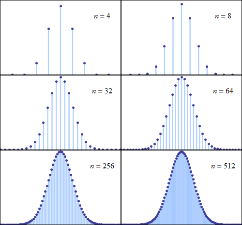
In probability theory, the de Moivre–Laplace theorem, which is a special case of the central limit theorem, states that the normal distribution may be used as an approximation to the binomial distribution under certain conditions. In particular, the theorem shows that the probability mass function of the random number of “successes” observed in a series of n independent Bernoulli trials, each having probability p of success (a binomial distribution with n trials), converges to the probability density function of the normal distribution with mean np and standard deviation √np(1-p), as n grows large, assuming p is not 0 or 1.
The theorem appeared in the second edition of The Doctrine of Chances by Abraham de Moivre, published in 1738. Although de Moivre did not use the term “Bernoulli trials”, he wrote about the probability distribution of the number of times “heads” appears when a coin is tossed 3600 times.[1]
This is one derivation of the particular Gaussian function used in the normal distribution.

Consider tossing a set of n coins a very large number of times and counting the number of “heads” that result each time. The possible number of heads on each toss, k, runs from 0 to n along the horizontal axis, while the vertical axis represents the relative frequency of occurrence of the outcome k heads. The height of each dot is thus the probability of observing k heads when tossing n coins (a binomial distribution based on n trials). According to the de Moivre–Laplace theorem, as n grows large, the shape of the discrete distribution converges to the continuous Gaussian curve of the normal distribution.
Theorem
As n grows large, for k in the neighborhood of np we can approximate[2][3]
in the sense that the ratio of the left-hand side to the right-hand side converges to 1 as n → ∞.
Proof
Note that k cannot be fixed or it would quickly fall outside the range of interest as n → ∞. What is needed is to let k vary but always be a fixed number of standard deviations from the mean, so that it is always associated with the same point on the standard normal distribution. We can do this by defining
for some fixed x. Then, for example, when x = 1, k will always be 1 standard deviation from the mean. From this definition we have the approximations as n → ∞.
However, the left-hand side requires that k be an integer. Keeping the notation but assuming that k is the nearest integer given by the definition, this is seen to be inconsequential in the limit by noting that as n → ∞ the change in x required to make k an integer becomes small and successive integer values of k produce converging values on the right-hand side:
The proof consists of transforming the left-hand side to the right-hand side by three approximations.
First, according to Stirling’s formula, we can replace the factorial of a large number n with the approximation:
Thus
Next, use the approximation to match the root above to the desired root on the right-hand side.
Finally, rewrite the expression as an exponential and use the Taylor Series approximation for ln(1+x):
Then
邏輯雖實真無欺,數大之美品嚐難,故有模擬加互動,

The Molecular Workbench is developed by the Concord Consortium. Learn about our work »
 Molecular Workbench was awarded the prestigious SPORE Prize Learn More »
願君目睹理念生。
.png)
.png)
疑問之來醞釀久,
吉布斯悖論
熱力學中的吉布斯悖論(又稱吉布斯悖論)是由美國物理學家約西亞·吉布斯提出來的。吉布斯悖論一直是統計力學和量子力學的學科發展中的一個重要議題。
混合當然是指不同物質的混合。相同的物質放在一起就不叫混合了。混合熵的計算數值是一定的,無論兩種物質 A 和 B 僅僅有些微差別還是差別很大。當兩種物質僅僅有些微差別時混合過程仍然有所謂混合熵。當兩種物質完全相同時混合熵的計算數值為零。混合熵隨A和B的相似程度的變化是不連續的。
對這個悖論的解釋是,當氣體不同時,不論其程度如何,原則上是有辦法把它分開的,因此混合有不可逆的擴散發生。但如果兩氣體本來就是一種氣體的兩部 分,則混合後是無法再分開復原的。因此在理論上並無矛盾。對吉布斯悖論中的混合熵隨A 和B的相似程度的變化的不連續性有多種解釋。
真要解吉布斯悖論就必須證明混合熵實際上是連續變化的。約翰·馮·諾伊曼 (John von Neumann)提出混合熵隨A和B的相似程度的變化而連續地變為零。
事物常有定見在。
Illustration of the problem
Gibbs himself considered the following problem that arises if the ideal gas entropy is not extensive.[1] Two identical containers of an ideal gas sit side-by-side. There is a certain amount of entropy S associated with each container of gas, and this depends on the volume of each container. Now a door in the container walls is opened to allow the gas particles to mix between the containers. No macroscopic changes occur, as the system is in equilibrium. The entropy of the gas in the two-container system can be easily calculated, but if the equation is not extensive, the entropy would not be 2S. In fact, the non-extensive entropy quantity defined and studied by Gibbs would predict additional entropy. Closing the door then reduces the entropy again to 2S, in supposed violation of the Second Law of Thermodynamics.
As understood by Gibbs,[2] and reemphasized more recently,[3][4] this is a misapplication of Gibbs’ non-extensive entropy quantity. If the gas particles are distinguishable, closing the doors will not return the system to its original state – many of the particles will have switched containers. There is a freedom in what is defined as ordered, and it would be a mistake to conclude the entropy had not increased. In particular, Gibbs’ non-extensive entropy quantity for an ideal gas was not intended for varying numbers of particles.
The paradox is averted by concluding the indistinguishability (at least effective indistinguishability) of the particles in the volume. This results in the extensive Sackur–Tetrode equation for entropy, as derived next.
或早萌芽正逢春!!
The mixing paradox
A closely related paradox to the Gibbs paradox is the mixing paradox. Again take a box with a partition in it, with gas A on one side, gas B on the other side, and both gases are at the same temperature and pressure. If gas A and B are different gases, there is an entropy that arises once the gases are mixed. If the gases are the same, no additional entropy is calculated. The additional entropy from mixing does not depend on the character of the gases; it only depends on the fact that the gases are different. The two gases may be arbitrarily similar, but the entropy from mixing does not disappear unless they are the same gas – a paradoxical discontinuity.
This “paradox” can be explained by carefully considering the definition of entropy. In particular, as concisely explained by Jaynes,[2] definitions of entropy are arbitrary
As a central example in Jaynes’ paper points out, one can develop a theory that treats two gases as similar even if those gases may in reality be distinguished through sufficiently detailed measurement. As long as we do not perform these detailed measurements, the theory will have no internal inconsistencies. (In other words, it does not matter that we call gases A and B by the same name if we have not yet discovered that they are distinct.) If our theory calls gases A and B the same, then entropy does not change when we mix them. If our theory calls gases A and B different, then entropy does increase when they are mixed. This insight suggests that the ideas of “thermodynamic state” and of “entropy” are somewhat subjective.
The differential increase in entropy (dS) as a result of mixing dissimilar gases, multiplied by the temperature (T), equals the minimum amount of work we must do to restore the gases to their original separated state. Suppose that two gases are different, but that we are unable to detect their differences. If these gases are in a box, segregated from one another by a partition, how much work does it take to restore the system’s original state after we remove the partition and let the gases mix?
None – simply reinsert the partition. Even though the gases have mixed, there was never a detectable change of state in the system, because by hypothesis the gases are experimentally indistinguishable.
As soon as we can distinguish the difference between gases, the work necessary to recover the pre-mixing macroscopic configuration from the post-mixing state becomes nonzero. This amount of work does not depend on how different the gases are, but only on whether they are distinguishable.
This line of reasoning is particularly informative when considering the concepts of indistinguishable particles and correct Boltzmann counting. Boltzmann’s original expression for the number of states available to a gas assumed that a state could be expressed in terms of a number of energy “sublevels” each of which contain a particular number of particles. While the particles in a given sublevel were considered indistinguishable from each other, particles in different sublevels were considered distinguishable from particles in any other sublevel. This amounts to saying that the exchange of two particles in two different sublevels will result in a detectably different “exchange macrostate” of the gas. For example, if we consider a simple gas with N particles, at sufficiently low density that it is practically certain that each sublevel contains either one particle or none (i.e. a Maxwell–Boltzmann gas), this means that a simple container of gas will be in one of N! detectably different “exchange macrostates”, one for each possible particle exchange.
Just as the mixing paradox begins with two detectably different containers, and the extra entropy that results upon mixing is proportional to the average amount of work needed to restore that initial state after mixing, so the extra entropy in Boltzmann’s original derivation is proportional to the average amount of work required to restore the simple gas from some “exchange macrostate” to its original “exchange macrostate”. If we assume that there is in fact no experimentally detectable difference in these “exchange macrostates” available, then using the entropy which results from assuming the particles are indistinguishable will yield a consistent theory. This is “correct Boltzmann counting”.
It is often said that the resolution to the Gibbs paradox derives from the fact that, according to the quantum theory, like particles are indistinguishable in principle. By Jaynes’ reasoning, if the particles are experimentally indistinguishable for whatever reason, Gibbs paradox is resolved, and quantum mechanics only provides an assurance that in the quantum realm, this indistinguishability will be true as a matter of principle, rather than being due to an insufficiently refined experimental capability.
這位傑尼斯
Edwin Thompson Jaynes
Edwin Thompson Jaynes (July 5, 1922 – April 30,[1] 1998) was the Wayman Crow Distinguished Professor of Physics at Washington University in St. Louis. He wrote extensively on statistical mechanics and on foundations of probability and statistical inference, initiating in 1957 the MaxEnt interpretation of thermodynamics,[2][3] as being a particular application of more general Bayesian/information theory techniques (although he argued this was already implicit in the works of Gibbs). Jaynes strongly promoted the interpretation of probability theory as an extension of logic.
───
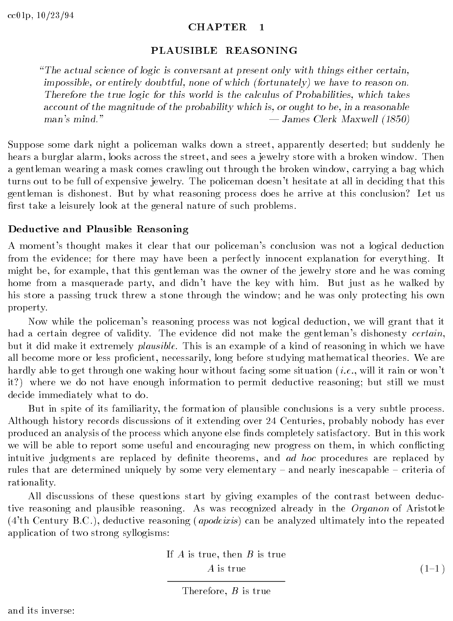
先生將波利亞之『似合理的』Plausible 『推理』系統化,
喬治‧波利亞
George Pólya
suggests the following steps when solving a mathematical problem:
1. First, you have to understand the problem.
2. After understanding, then make a plan.
3. Carry out the plan.
4. Look back on your work. How could it be better?
If this technique fails, Pólya advises: “If you can’t solve a problem, then there is an easier problem you can solve: find it.” Or: “If you cannot solve the proposed problem, try to solve first some related problem. Could you imagine a more accessible related problem?”
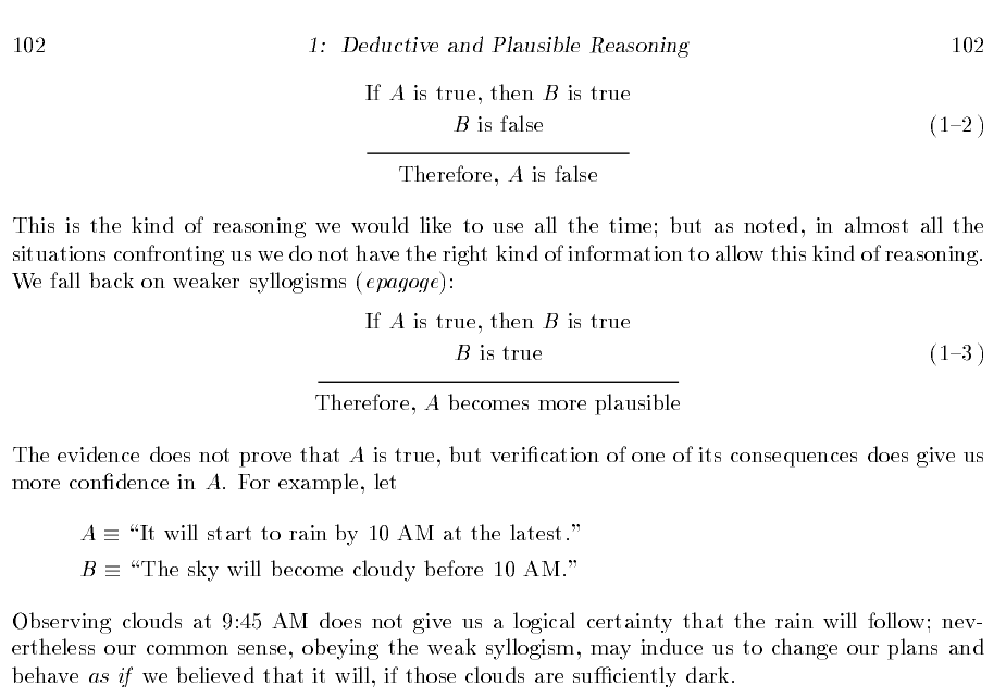
喬治‧波利亞長期從事數學教學,對數學思維的一般規律有深入的研究,一生推動數學教育。一九五四年,波利亞寫了兩卷不同於一般的數學書《Induction And_Analogy In Mathematics》與《Patterns Of Plausible Inference》探討『啟發式』之『思維樣態』,這常常是一種《數學發現》之切入點,也是探尋『常識徵候』中的『合理性』根源。舉個例子來說,典型的亞里斯多德式的『三段論』 syllogisms ︰
![]()
![]() 真,
真, ![]() 真。
真。
如果對比著『似合理的』Plausible 『推理』︰
![]()
![]() 真,
真, ![]() 更可能是真。
更可能是真。
這種『推理』一般稱之為『肯定後件』 ![]() 的『邏輯誤謬』。因為在『邏輯』上,這種『形式』的推導,並不『必然的』保障『歸結』一定是『真』的。然而這種『推理形式』是完全沒有『道理』的嗎?如果從『三段論』之『邏輯』上來講,要是
的『邏輯誤謬』。因為在『邏輯』上,這種『形式』的推導,並不『必然的』保障『歸結』一定是『真』的。然而這種『推理形式』是完全沒有『道理』的嗎?如果從『三段論』之『邏輯』上來講,要是 ![]() 為『假』,
為『假』,![]() 也就『必然的』為『假』。所以假使
也就『必然的』為『假』。所以假使 ![]() 為『真』之『必要條件』
為『真』之『必要條件』 ![]() 為『真』,那麼
為『真』,那麼 ![]() 不該是『更可能』是『真』的嗎??
不該是『更可能』是『真』的嗎??
─── 摘自《物理哲學·下中……》
把『機率論』帶入邏輯殿堂,
Probability Theory: The Logic Of Science
he material available from this page is a pdf version of E.T. Jaynes’s book.
Introduction
Please note that the contents of the file from the link below is slightly of out sync with the actual contents of the book. The listing on this page correspond to the existing chapter order and names.
……


───
誠非偶然的耶!!??若是人人都能如是『運作理則』,庶幾可免『賭徒謬誤』矣??!!
── 摘自《W!o+ 的《小伶鼬工坊演義》︰神經網絡【學而堯曰】七》


