身處將入『人工智慧』之時代,假使不能善用『軟體工具』,豈非落伍?若說非不能也!年少未曾學也!!當思活到老學到老乎??由於這個系列文章將用到
‧ SciPy
‧ NumPy & SymPy
‧ …
尤其是『SymPy』,它們的『安裝』、『說明』與『範例』或不宜多所剪貼,故請舊雨新知參閱相關鍊結以及所屬文本哩。
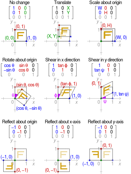
這裡摘要只為方便讀者回顧『矩陣運算』︰
翻古出新,談談如何用『SymPy』之
‧ Matrices
‧ Matrices (linear algebra)
模組為『工具』,操作
線性代數中,初等矩陣(又稱為基本矩陣[1])是一個與單位矩陣只有微小區別的矩陣。具體來說,一個n階單位矩陣E經過一次初等行變換或一次初等列變換所得矩陣稱為n階初等矩陣。[2]
操作
初等矩陣分為3種類型,分別對應著3種不同的行/列變換。
- 兩行(列)互換:
-

- 把某行(列)乘以一非零常數:
 其中
其中 
- 把第i行(列)加上第j行(列)的k倍:

初等矩陣即是將上述3種初等變換應用於一單位矩陣的結果。以下只討論對某行的變換,列變換可以類推。
行互換
這一變換Tij,將一單位矩陣的第i行的所有元素與第j行互換。

性質
-
- 逆矩陣即自身:
 。
。
- 因為單位矩陣的行列式為1,故
 。與其他相同大小的方陣A亦有一下性質:
  。
。
把某行乘以一非零常數
這一變換Ti(m),將第i行的所有元素乘以一非零常數m。

性質
-
- 逆矩陣為
 。
。
- 此矩陣及其逆矩陣均為對角矩陣。
- 其行列式
 。故對於一等大方陣A有
  。
。
把第i行加上第j行的m倍
這一變換Tij(m),將第i行加上第j行的m倍。

性質
-
- 逆矩陣具有性質
 。
。
- 此矩陣及其逆矩陣均為三角矩陣。
 。故對於一等大方陣A有:
  。
。
親自『實證』消去法的精神,體驗用『工具』來『學習』之樂趣吧! !
省思這個『初等』當真可『模擬』紙筆運算嗎??
pi@raspberrypi:~ *** QuickLaTeX cannot compile formula:
python3
Python 3.4.2 (default, Oct 19 2014, 13:31:11)
[GCC 4.9.1] on linux
Type "help", "copyright", "credits" or "license" for more information.
>>> from sympy import *
>>> init_printing()
>>> a, b, c, d, e, f, g, h, i, m = symbols('a, b, c, d, e, f, g, h, i, m')
>>> M = Matrix([[a, b, c], [d, e, f], [g, h, i]])
>>> M
⎡a b c⎤
⎢ ⎥
⎢d e f⎥
⎢ ⎥
⎣g h i⎦
>>> 二三列交換 = Matrix([[1, 0, 0], [0, 0, 1], [0, 1, 0]])
>>> 二三列交換
⎡1 0 0⎤
⎢ ⎥
⎢0 0 1⎥
⎢ ⎥
⎣0 1 0⎦
>>> 二三列交換 * M
⎡a b c⎤
⎢ ⎥
⎢g h i⎥
⎢ ⎥
⎣d e f⎦
>>> 第二列乘m = Matrix([[1, 0, 0], [0, m, 0], [0, 0, 1]])
>>> 第二列乘m
⎡1 0 0⎤
⎢ ⎥
⎢0 m 0⎥
⎢ ⎥
⎣0 0 1⎦
>>> 第二列乘m * M
⎡ a b c ⎤
⎢ ⎥
⎢d⋅m e⋅m f⋅m⎥
⎢ ⎥
⎣ g h i ⎦
>>> 第三列加第二列乘m = Matrix([[1, 0, 0], [0, 1, 0], [0, m, 1]])
>>> 第三列加第二列乘m
⎡1 0 0⎤
⎢ ⎥
⎢0 1 0⎥
⎢ ⎥
⎣0 m 1⎦
>>> 第三列加第二列乘m * M
⎡ a b c ⎤
⎢ ⎥
⎢ d e f ⎥
⎢ ⎥
⎣d⋅m + g e⋅m + h f⋅m + i⎦
>>>
</pre>
<span style="color: #003300;">或可得『自學』之法哩!!??</span>
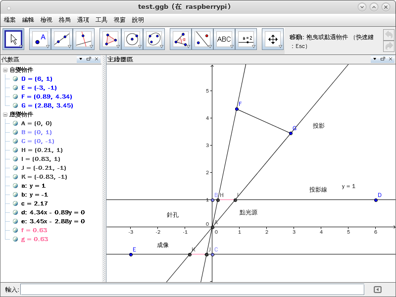
─── 摘自《<a href="http://www.freesandal.org/?p=56412">光的世界︰派生科學計算三</a>》
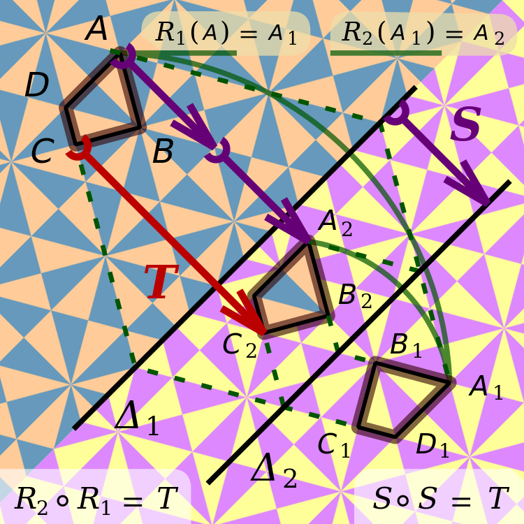
<span style="color: #666699;">重溫『仿射變換』︰</span>
<span style="color: #808080;">廬山東林寺<a style="color: #808080;" href="http://www.freesandal.org/?p=2711">三笑庭</a>名聯‧清‧唐蝸寄</span>
<span style="color: #808080;">橋跨虎溪,三教三源流,三人三笑語;</span>
<span style="color: #808080;"> 蓮開僧舍,一花一世界,一葉一如來。</span>
<span style="color: #003300;">曾經三人三笑語,聞得虎嘯,恍然大悟。何故三詠三抒懷︰</span>
<div class="wc-shortcodes-row wc-shortcodes-item wc-shortcodes-clearfix"><div class="wc-shortcodes-column wc-shortcodes-content wc-shortcodes-one-half wc-shortcodes-column-first ">
<span style="color: #808080;"><a style="color: #808080;" href="https://zh.wikisource.org/zh-hant/%E8%A9%A0%E4%BA%8C%E7%96%8F">詠二疏</a>‧陶淵明</span>
<span style="color: #808080;">大象轉四時,功成者自去。</span>
<span style="color: #808080;"> 借問衰周來,幾人得其趣?</span>
<span style="color: #808080;"> 遊目漢廷中,二疏復此舉。</span>
<span style="color: #808080;"> 高嘯返舊居,長揖儲君傅。</span>
<span style="color: #808080;"> 餞送傾皇朝,華軒盈道路。</span>
<span style="color: #808080;"> 離別情所悲,余榮何足顧!</span>
<span style="color: #808080;"> 事勝感行人,賢哉豈常譽?</span>
<span style="color: #808080;"> 厭厭閭裏歡,所營非近務。</span>
<span style="color: #808080;"> 促席延故老,揮觴道平素。</span>
<span style="color: #808080;"> 問金終寄心,清言曉未悟。</span>
<span style="color: #808080;"> 放意樂餘年,遑恤身後慮。</span>
<span style="color: #808080;"> 誰雲其人亡,久而道彌著。</span>
</div><div class="wc-shortcodes-column wc-shortcodes-content wc-shortcodes-one-half wc-shortcodes-column-last ">
<span style="color: #808080;"><a style="color: #808080;" href="https://zh.wikisource.org/zh-hant/%E8%A9%A0%E4%B8%89%E8%89%AF">詠三良</a>‧陶淵明</span>
<span style="color: #808080;">彈冠乘通津,但懼時我遺;</span>
<span style="color: #808080;"> 服勤盡歲月,常恐功愈微。</span>
<span style="color: #808080;"> 忠情謬獲露,遂為君所私。</span>
<span style="color: #808080;"> 出則陪文輿,入必侍丹帷;</span>
<span style="color: #808080;"> 箴規向已從,計議初無虧。</span>
<span style="color: #808080;"> 一朝長逝後,願言同此歸。</span>
<span style="color: #808080;"> 厚恩因難忘,君命安可違?</span>
<span style="color: #808080;"> 臨穴罔惟疑,投義誌攸希。</span>
<span style="color: #808080;"> 荊棘籠高墳,黃鳥聲正悲。</span>
<span style="color: #808080;"> 良人不可贖,泫然沾我衣。</span>
</div></div>
<span style="color: #808080;"><a style="color: #808080;" href="https://zh.wikisource.org/zh-hant/%E8%A9%A0%E8%8D%8A%E8%BB%BB">詠荊軻</a>‧陶淵明</span>
<span style="color: #808080;">燕丹善養士,誌在報強嬴。</span>
<span style="color: #808080;"> 招集百夫良,歲暮得荊卿。</span>
<span style="color: #808080;"> 君子死知己,提劍出燕京;</span>
<span style="color: #808080;"> 素驥鳴廣陌,慷慨送我行。</span>
<span style="color: #808080;"> 雄發指危冠,猛氣衝長纓。</span>
<span style="color: #808080;"> 飲餞易水上,四座列群英。</span>
<span style="color: #808080;"> 漸離擊悲筑,宋意唱高聲。</span>
<span style="color: #808080;"> 蕭蕭哀風逝,淡淡寒波生。</span>
<span style="color: #808080;"> 商音更流涕,羽奏壯士驚。</span>
<span style="color: #808080;"> 心知去不歸,且有後世名。</span>
<span style="color: #808080;"> 登車何時顧,飛蓋入秦庭。</span>
<span style="color: #808080;"> 淩厲越萬裏,逶迤過千城。</span>
<span style="color: #808080;"> 圖窮事自至,豪主正怔營。</span>
<span style="color: #808080;"> 惜哉劍術疏,奇功遂不成!</span>
<span style="color: #808080;"> 其人雖已沒,千載有餘情。</span>
<span style="color: #003300;">晉時<a style="color: #003300;" href="https://zh.wikipedia.org/zh-tw/%E9%99%B6%E6%B8%8A%E6%98%8E">淵明</a>,晉後名潛,已棄五斗米,不知姓字忘其何人,<a style="color: #003300;" href="http://www.freesandal.org/?p=29427">五柳先生</a>『伍』『柳』吟誦耶??果真二三子其志一也!!雖說是移時隔空得失不同,其人其心何其相似乎??!!先生『<a style="color: #003300;" href="http://www.zwbk.org/MyLemmaShow.aspx?zh=zh-tw&lid=78693">菀柳</a>』之『情』仍一樣吧!!??</span>
<span style="color: #808080;">誰雲其人亡,久而道彌著。</span>
<span style="color: #808080;">良人不可贖,泫然沾我衣。</span>
<span style="color: #808080;">其人雖已沒,千載有餘情。</span>
大暑已過,入秋之際,講此『春耕夏耘』之『心法』勒。古今中外『學問』縱有千百種,談起功夫『心法』則一矣。往往其『志一』其『人同』也!!只是『一花』『一葉』真誠對待歟??
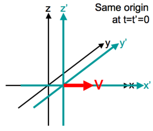
<span style="color: #003300;">如果天地公平,天理能隨觀者變乎??故知物理學之所以著意於</span>
<span style="color: #003300;"><a style="color: #003300;" href="https://zh.wikipedia.org/zh-tw/%E4%BB%BF%E5%B0%84%E5%8F%98%E6%8D%A2">仿射變換</a>之<span id=".E6.80.A7.E8.B3.AA" class="mw-headline">性質</span>了!!</span>
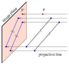
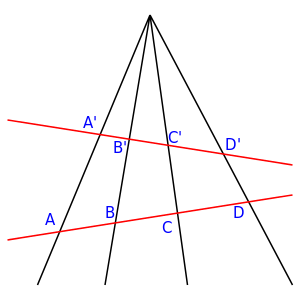
<span style="color: #808080;">一仿射變換保留了:</span>
<ol>
<li><span style="color: #808080;">點之間的共線性,例如通過同一線之點 (即稱為共線點)在變換後仍呈共線。</span></li>
<li><span style="color: #808080;">向量沿著一線的比例,例如對相異共線三點 <img class="mwe-math-fallback-image-inline" src="https://wikimedia.org/api/rest_v1/media/math/render/svg/34ca63f1bf90ff180f60ae1921599052c62afe89" alt="p_{1},\,p_{2},\,p_{3}," width="98" height="19" /> <img class="mwe-math-fallback-image-inline" src="https://wikimedia.org/api/rest_v1/media/math/render/svg/033ae99f7900d8c5bd3459a80f9e7f5f6fb07791" alt="\overrightarrow {p_{1}p_{2}}" width="40" height="30" /> 與 <img class="mwe-math-fallback-image-inline" src="https://wikimedia.org/api/rest_v1/media/math/render/svg/a5f97fcb4b346ff107baa509e1aebac328e8bd4b" alt="\overrightarrow {p_{2}p_{3}}" width="42" height="32" />的比例同於 <img class="mwe-math-fallback-image-inline" src="https://wikimedia.org/api/rest_v1/media/math/render/svg/a49164cfaadf80350914df400643af54e7bae911" alt="\overrightarrow {f(p_{1})f(p_{2})}" width="96" height="39" />及<span class="mwe-math-mathml-inline mwe-math-mathml-a11y"> </span><img class="mwe-math-fallback-image-inline" src="https://wikimedia.org/api/rest_v1/media/math/render/svg/475803f6b965c1a6cc97f28c43df6a0430d3512c" alt="\overrightarrow {f(p_{2})f(p_{3})}" width="104" height="42" />。</span></li>
<li><span style="color: #808080;">帶不同質量的點之<a style="color: #808080;" title="質心" href="https://zh.wikipedia.org/wiki/%E8%B3%AA%E5%BF%83">質心</a>。</span></li>
</ol>
<span style="color: #808080;">一仿射變換為可逆的<a class="mw-redirect" style="color: #808080;" title="若且唯若" href="https://zh.wikipedia.org/wiki/%E8%8B%A5%E4%B8%94%E5%94%AF%E8%8B%A5">若且唯若</a>A為可逆的。在矩陣表示中,其反元素為</span>
<dl>
<dd><span style="color: #808080;"><img class="mwe-math-fallback-image-inline" src="https://wikimedia.org/api/rest_v1/media/math/render/svg/ddfc76aceafb89584e37d908a18bb693a77e64c7" alt="{\begin{bmatrix}A^{{-1}}&-A^{{-1}}{\vec {b}}\ \\0,\ldots ,0&1\end{bmatrix}}" width="207" height="65" /></span></dd>
</dl>
<span style="color: #808080;">可逆仿射變換組成<a class="new" style="color: #808080;" title="仿射群(頁面不存在)" href="https://zh.wikipedia.org/w/index.php?title=%E4%BB%BF%E5%B0%84%E7%BE%A4&action=edit&redlink=1">仿射群</a>,其中包含具n階的<a class="mw-redirect" style="color: #808080;" title="一般線性群" href="https://zh.wikipedia.org/wiki/%E4%B8%80%E8%88%AC%E7%B7%9A%E6%80%A7%E7%BE%A4">一般線性群</a>為子群,且自身亦為一n+1階的一般線性群之子群。 當A為常數乘以<a style="color: #808080;" title="正交矩陣" href="https://zh.wikipedia.org/wiki/%E6%AD%A3%E4%BA%A4%E7%9F%A9%E9%98%B5">正交矩陣</a>時,此子集合構成一子群,稱之為<a style="color: #808080;" title="相似 (幾何)" href="https://zh.wikipedia.org/wiki/%E7%9B%B8%E4%BC%BC_%28%E5%B9%BE%E4%BD%95%29">相似變換</a>。<span style="color: #ff9900;">舉例而言,假如仿射變換於一平面上且假如A之<a style="color: #ff9900;" title="行列式" href="https://zh.wikipedia.org/wiki/%E8%A1%8C%E5%88%97%E5%BC%8F">行列式</a>為1或-1,那麼該變換即為<a class="new" style="color: #ff9900;" title="等面積變換(頁面不存在)" href="https://zh.wikipedia.org/w/index.php?title=%E7%AD%89%E9%9D%A2%E7%A9%8D%E8%AE%8A%E6%8F%9B&action=edit&redlink=1">等面積變換</a>。此類變換組成一稱為等仿射群的子集。一同時為等面積變換與相似變換之變換,即為一平面上保持<a class="mw-redirect" style="color: #ff9900;" title="歐幾里德距離" href="https://zh.wikipedia.org/wiki/%E6%AC%A7%E5%87%A0%E9%87%8C%E5%BE%B7%E8%B7%9D%E7%A6%BB">歐幾里德距離</a>不變之<a style="color: #ff9900;" title="等距同構" href="https://zh.wikipedia.org/wiki/%E7%AD%89%E8%B7%9D%E5%90%8C%E6%9E%84">保距映射</a>。</span> 這些群都有一保留了原<a style="color: #808080;" title="定向 (向量空間)" href="https://zh.wikipedia.org/wiki/%E5%AE%9A%E5%90%91_%28%E5%90%91%E9%87%8F%E7%A9%BA%E9%96%93%29">定向</a>的子群,也就是其對應之<i>A</i>的行列式大於零。在最後一例中,即為三維中<a class="mw-redirect" style="color: #808080;" title="剛體" href="https://zh.wikipedia.org/wiki/%E5%89%9B%E9%AB%94">剛體</a>運動之群(旋轉加平移)。 假如有一不動點,我們可以將其當成原點,則仿射變換被縮還到一線性變換。這使得變換更易於分類與理解。舉例而言,將一變換敘述為特定軸的旋轉,相較於將其形容為平移與旋轉的結合,更能提供變換行為清楚的解釋。只是,這取決於應用與內容。</span>
<span style="color: #003300;">若知『平移』與『旋轉』為『保距映射』,餘理可知矣︰</span>
<span style="color: #808080;">※矩陣乘法不具『交換性』,正是『平移』後『旋轉』往往不等於『旋轉』再『平移』也。</span>
<pre class="lang:python decode:true ">pi@raspberrypi:~
*** Error message:
Missing $ inserted.
Missing $ inserted.
leading text: >>> init_
Unicode character ⎡ (U+23A1)
leading text: ⎡
Unicode character ⎤ (U+23A4)
leading text: ⎡a b c⎤
Unicode character ⎢ (U+23A2)
leading text: ⎢
Unicode character ⎥ (U+23A5)
leading text: ⎢ ⎥
Unicode character ⎢ (U+23A2)
leading text: ⎢
Unicode character ⎥ (U+23A5)
leading text: ⎢d e f⎥
Unicode character ⎢ (U+23A2)
leading text: ⎢
Unicode character ⎥ (U+23A5)
leading text: ⎢ ⎥
Unicode character ⎣ (U+23A3)
leading text: ⎣
Unicode character ⎦ (U+23A6)
leading text: ⎣g h i⎦
Missing $ inserted.
Unicode character 二 (U+4E8C)
leading text: >>> 二
Unicode character 三 (U+4E09)
leading text: >>> 二三
Unicode character 列 (U+5217)
ipython3
Python 3.4.2 (default, Oct 19 2014, 13:31:11)
Type "copyright", "credits" or "license" for more information.
IPython 2.3.0 -- An enhanced Interactive Python.
? -> Introduction and overview of IPython's features.
%quickref -> Quick reference.
help -> Python's own help system.
object? -> Details about 'object', use 'object??' for extra details.
In [1]: from sympy import *
In [2]: init_printing()
In [3]: xα, yα, xβ, yβ, Tx, Ty, θ = symbols('xα, yα, xβ, yβ, Tx, Ty, θ')
In [4]: T = Matrix([[1, 0, Tx], [0, 1, Ty], [0, 0, 1]])
In [5]: T
Out[5]:
⎡1 0 Tx⎤
⎢ ⎥
⎢0 1 Ty⎥
⎢ ⎥
⎣0 0 1 ⎦
In [6]: T.det()
Out[6]: 1
In [7]: R = Matrix([[cos(θ), sin(θ), 0], [-sin(θ), cos(θ), 0], [0, 0, 1]])
In [8]: R
Out[8]:
⎡cos(θ) sin(θ) 0⎤
⎢ ⎥
⎢-sin(θ) cos(θ) 0⎥
⎢ ⎥
⎣ 0 0 1⎦
In [9]: R.det()
Out[9]:
2 2
sin (θ) + cos (θ)
In [10]: R.det().simplify()
Out[10]: 1
In [11]: α平移 = T * Matrix([xα, yα, 1])
In [12]: α平移
Out[12]:
⎡Tx + xα⎤
⎢ ⎥
⎢Ty + yα⎥
⎢ ⎥
⎣ 1 ⎦
In [13]: β平移 = T * Matrix([xβ, yβ, 1])
In [14]: β平移
Out[14]:
⎡Tx + xβ⎤
⎢ ⎥
⎢Ty + yβ⎥
⎢ ⎥
⎣ 1 ⎦
In [15]: αβ平移距離 = (α平移[0] - β平移[0])** 2 + (α平移[1] - β平移[1])** 2
In [16]: αβ平移距離
Out[16]:
2 2
(xα - xβ) + (yα - yβ)
In [17]: α旋轉 = R * Matrix([xα, yα, 1])
In [18]: α旋轉
Out[18]:
⎡xα⋅cos(θ) + yα⋅sin(θ) ⎤
⎢ ⎥
⎢-xα⋅sin(θ) + yα⋅cos(θ)⎥
⎢ ⎥
⎣ 1 ⎦
In [19]: β旋轉 = R * Matrix([xβ, yβ, 1])
In [20]: β旋轉
Out[20]:
⎡xβ⋅cos(θ) + yβ⋅sin(θ) ⎤
⎢ ⎥
⎢-xβ⋅sin(θ) + yβ⋅cos(θ)⎥
⎢ ⎥
⎣ 1 ⎦
In [21]: αβ旋轉距離 = (α旋轉[0] - β旋轉[0])** 2 + (α旋轉[1] - β旋轉[1])** 2
In [22]: αβ旋轉距離
Out[22]:
2
(-xα⋅sin(θ) + xβ⋅sin(θ) + yα⋅cos(θ) - yβ⋅cos(θ)) + (xα⋅cos(θ) - xβ⋅cos(θ) + y
2
α⋅sin(θ) - yβ⋅sin(θ))
In [23]: αβ旋轉距離.expand().simplify()
Out[23]:
2 2 2 2
xα - 2⋅xα⋅xβ + xβ + yα - 2⋅yα⋅yβ + yβ
In [24]: R*T
Out[24]:
⎡cos(θ) sin(θ) Tx⋅cos(θ) + Ty⋅sin(θ) ⎤
⎢ ⎥
⎢-sin(θ) cos(θ) -Tx⋅sin(θ) + Ty⋅cos(θ)⎥
⎢ ⎥
⎣ 0 0 1 ⎦
In [25]: T*R
Out[25]:
⎡cos(θ) sin(θ) Tx⎤
⎢ ⎥
⎢-sin(θ) cos(θ) Ty⎥
⎢ ⎥
⎣ 0 0 1 ⎦
In [26]:
─── 摘自《光的世界︰派生科學計算六‧下》
特別點出

As shown above, an affine map is the composition of two functions: a translation and a linear map. Ordinary vector algebra uses matrix multiplication to represent linear maps, and vector addition to represent translations. Formally, in the finite-dimensional case, if the linear map is represented as a multiplication by a matrix  and the translation as the addition of a vector
  , an affine map
  acting on a vector
  can be represented as
-

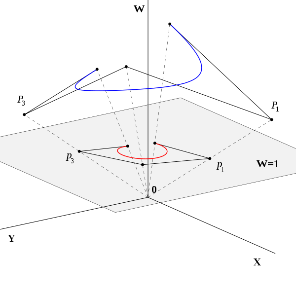
Augmented matrix
Using an augmented matrix and an augmented vector, it is possible to represent both the translation and the linear map using a single matrix multiplication. The technique requires that all vectors are augmented with a “1” at the end, and all matrices are augmented with an extra row of zeros at the bottom, an extra column—the translation vector—to the right, and a “1” in the lower right corner. If is a matrix,
-
![{\begin{bmatrix}{\vec {y}}\\1\end{bmatrix}}=\left[{\begin{array}{ccc|c}\,&A&&{\vec {b}}\ \\0&\ldots &0&1\end{array}}\right]{\begin{bmatrix}{\vec {x}}\\1\end{bmatrix}}](https://wikimedia.org/api/rest_v1/media/math/render/svg/4b3f8dfb50a5d0500891ce899036d73cfd362042)
is equivalent to the following
-

The above-mentioned augmented matrix is called an affine transformation matrix, or projective transformation matrix (as it can also be used to perform projective transformations).
This representation exhibits the set of all invertible affine transformations as the semidirect product of  and
and  . This is a group under the operation of composition of functions, called the affine group.
Ordinary matrix-vector multiplication always maps the origin to the origin, and could therefore never represent a translation, in which the origin must necessarily be mapped to some other point. By appending the additional coordinate “1” to every vector, one essentially considers the space to be mapped as a subset of a space with an additional dimension. In that space, the original space occupies the subset in which the additional coordinate is 1. Thus the origin of the original space can be found at  . A translation within the original space by means of a linear transformation of the higher-dimensional space is then possible (specifically, a shear transformation). The coordinates in the higher-dimensional space are an example of homogeneous coordinates. If the original space is Euclidean, the higher dimensional space is a real projective space.
The advantage of using homogeneous coordinates is that one can combine any number of affine transformations into one by multiplying the respective matrices. This property is used extensively in computer graphics, computer vision and robotics.
揣想『齊次座標系』擴充後之『加‧乘』『次序』吧◎
畢竟『理解』的目前是『人』耶◎
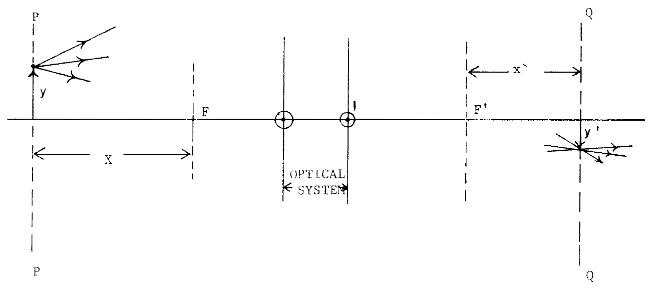

 是正或是負,
  都是正的也!如是對凸透鏡來講,無窮遠之物
  ,將成像於後焦點之平面上
  。那麼對凹透鏡來說,分明數學式子一樣!!又怎麼能一樣的呢??假使知道凹透鏡的後焦距面在凹透鏡之前,前焦距面在凹透鏡之後 ,能否釋疑呢???當真成像還是在後焦距面上!!!
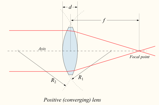


 表示物距
表示物距  比等效焦距大,但是很接近那個焦距。
 表達物距
表達物距 

 的啊??倘以現象而言,同也。皆平行光罷了!!
 向凸透鏡之前焦距趨近,其像距
  將由後焦距往後遠離,當
  ,像將在無窮遠也
  ,豈非透鏡後之平行光耶?★要是它從凸透鏡之主平面向後開始靠近前焦距面
  ,那麼
,那麼  ,難到能不是以『所見』為重,省略其透鏡後已然平行的乎!☆
 凹凸鏡面上之理耶☆
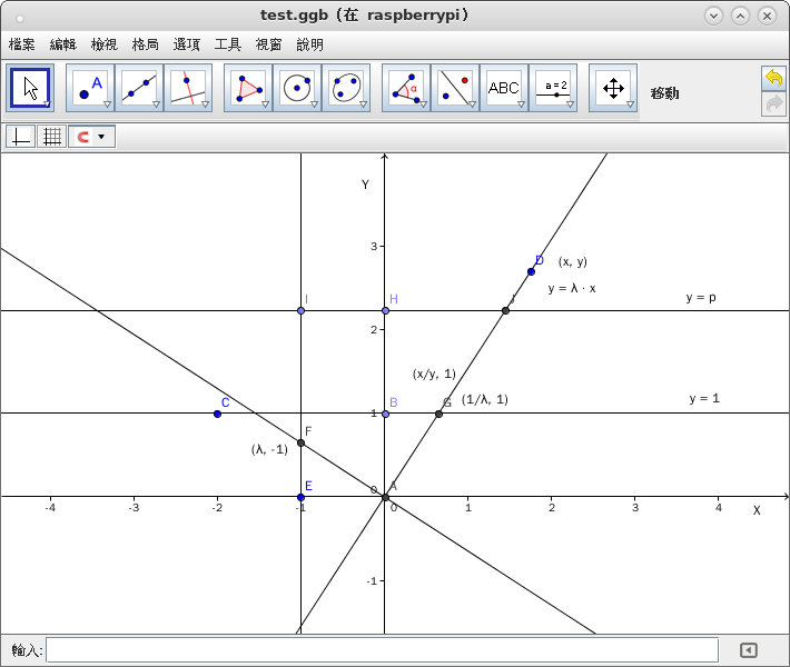
 是『點投派』一『投影函數』,那麼
 點上。難到
點上。難到  能夠『不等於』
  乎?
乎? 哩??
哩??

 這條『特殊線』的『交點』為『模型』哩?所謂的『無窮遠點』在哪裡?它有沒有『消失點』耶?…

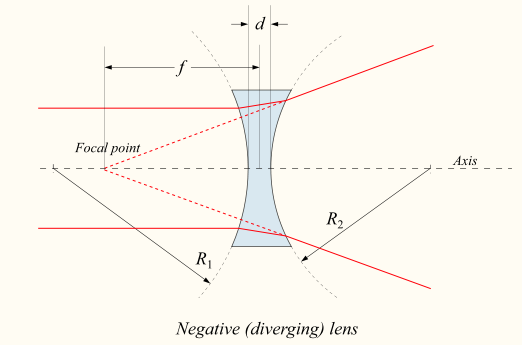
 、
、  的折射推導出
![\Phi (R_1, R_2) = \frac{1}{f} = (n-1) \left[ \frac{1}{R_1} - \frac{1}{R_2} \right]](http://www.freesandal.org/wp-content/ql-cache/quicklatex.com-c786934eb649a711256ab841df2bc7f1_l3.png "Rendered by QuickLaTeX.com")
 的反對稱性︰
 反轉成
反轉成  時,凹面將變凸面、凸面將變凹面,此時
  、
、  。事實上由於薄透鏡的特殊矩陣形制,兩個緊貼之薄透鏡組合還滿足交換律的哩︰

 。
。 參數等於
參數等於  。
。 之定義,可將之改寫為︰
 。
。
 ,但如成像落在下個薄透鏡之內,那麼
  ,於是正負與虛實之理相互爭勝, 用前一薄透鏡定之哉 ?或以後一薄透鏡定之哉!還是由薄透鏡組合定之哉??!!設若將此議論用之於像,豈不依然焉!!??奈何懷疑人眼或鏡頭只見虛像或實像呢★?倘已成像,就 是看到像了吧,又怎能不實的哩 。此時所謂設備之有無,難到不祇是為方不方便觀物的嗎☆!
![[x_1 : x_2]](https://wikimedia.org/api/rest_v1/media/math/render/svg/09404e16ef9ccccd05414dabeedac84b306fe9e4)
![[x_{1}:x_{2}]\sim [\lambda x_{1}:\lambda x_{2}].](https://wikimedia.org/api/rest_v1/media/math/render/svg/0e149dfacd2fd2bfcc157bc3da4e654227498373)
![\left\{[x : 1] \in \mathbf P^1(K) \mid x \in K\right\}.](https://wikimedia.org/api/rest_v1/media/math/render/svg/086c5d6b3f2d24eccfa35f0847c01d70c75b8c57)
![\infty = [1 : 0].](https://wikimedia.org/api/rest_v1/media/math/render/svg/54a6746d720a3849c5aeeeb5b0cb7fb0f12eac33)


![[x_1 : x_2] + [y_1 : y_2] = [x_1 y_2 + y_1 x_2 : x_2 y_2],](https://wikimedia.org/api/rest_v1/media/math/render/svg/94336d2523cfacf85e317a6516fe913cf0e030fd)
![[x_1 : x_2] \cdot [y_1 : y_2] = [x_1 y_1 : x_2 y_2],](https://wikimedia.org/api/rest_v1/media/math/render/svg/94fa88c74d83459420ba532b4549908fd14cbab9)
![[x_1 : x_2]^{-1} = [x_2 : x_1].](https://wikimedia.org/api/rest_v1/media/math/render/svg/c8afadaa9e638cbce6c51e27ae575b77755bc3cc)


![f_P \colon [\ell] \mapsto [m]](https://wikimedia.org/api/rest_v1/media/math/render/svg/0e04d1a74b6fa3b728499e363eb7ac0b25c08393)

![f_P (f_P (X)) = X \text{ for all }X \in [\ell]](https://wikimedia.org/api/rest_v1/media/math/render/svg/8b1a2bb9dee33511a3eea59395c7d55942a4275b)

 is the set of all lines in
  passing through the origin.
 and
and  are two nonzero vectors lying on the same line through the origin, then they are multiples of each other. This remark allows us to redefine
  as the quotient of
  by the equivalence relation
  (or
(or  ) if
) if 
 be the slope of the line
  passing through the origin and let
 equals
  .
. .
.
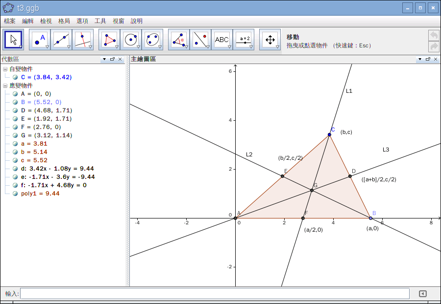
 三個參數?即使在思考過
  是『底』之『長』,
  是此『底』之『高』,
  是此『高』距與此『底』一端的距離。我們深信這就『確定』了那個三角形。然而若再問︰如果此三角形的三個頂點用更一般的
  、
、  、
、  來表達 ,如是分明有六個參數。那麼這兩種『表述』當真是一樣的嗎?設想你在桌面上『移動』一個三角形,從此『位置』此『方位』到達彼『位置』彼『方位』,你會認 為這個三角形『改變』了嗎??假使『直覺』以為『不變』,這個三角形就必得有使之『不變』的『因由』,這個『因由』不必『參照』解析幾何的『座標』而確立 。或可說它就是歐式幾何一個三角形的『定義』內涵而已。如此而言,一個『確定』的三角形,可由它的三個『邊長』來『確立』,所以六個參數補之以三個確定之 邊長關係,豈非還是三個參數的耶??