要是不能將相關的『概念』編織『成網』,使之上下聯繫、四通八達,思慮恐泥也!
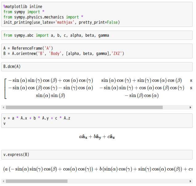
舉例來說︰如何求旋轉矩陣 


的旋轉軸呢?
或曰可用『本徵值方程式』  解之乎??
解之乎??
那麼一位親力親為者將可體驗頭暈腦脹呦!!
此處作者假借 SymPy 符號算術略釋此法︰

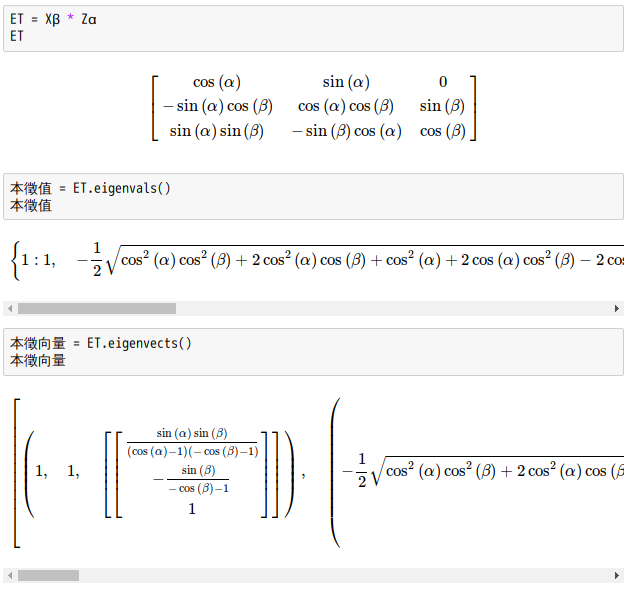
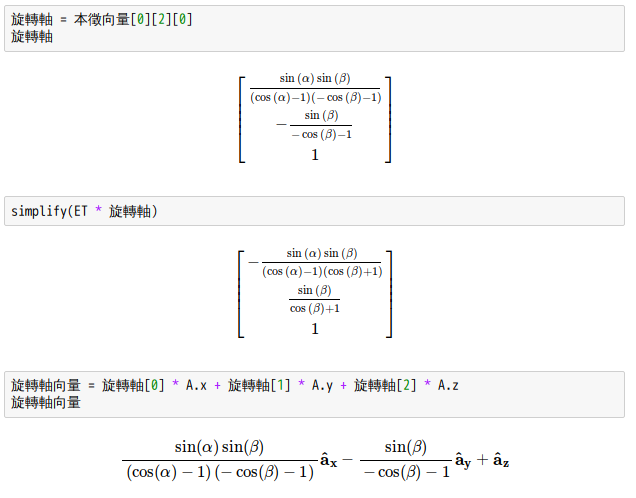
※ 所以用二『歐拉角』不用全,蓋不知 SymPy 要算多久故。
如是一個知道

的人,深入
Skew-symmetric matrix
In mathematics, particularly in linear algebra, a skew-symmetric (or antisymmetric or antimetric[1]) matrix is a square matrix whose transpose equals its negative; that is, it satisfies the condition
- AT = −A.
In terms of the entries of the matrix, if aij denotes the entry in the i th row and j th column; i.e., A = (aij), then the skew-symmetric condition is aji = −aij. For example, the following matrix is skew-symmetric:

-
Properties
Throughout, we assume that all matrix entries belong to a field
 whose characteristic is not equal to 2: that is, we assume that 1 + 1 ≠ 0, where 1 denotes the multiplicative identity and 0 the additive identity of the given field. If the characteristic of the field is 2, then a skew-symmetric matrix is the same thing as a symmetric matrix.
- The sum of two skew-symmetric matrices is skew-symmetric.
- A scalar multiple of a skew-symmetric matrix is skew-symmetric.
- The elements on the diagonal of a skew-symmetric matrix are zero, and therefore also its trace.
- If
 is a skew-symmetric matrix with real entries, i.e., if
  .
. - If is a real skew-symmetric matrix and
 is a real eigenvalue, then
  .
. - If is a real skew-symmetric matrix, then
 is invertible, where
  is the identity matrix.
Vector space structure
As a result of the first two properties above, the set of all skew-symmetric matrices of a fixed size forms a vector space. The space of
 skew-symmetric matrices has dimension n(n−1)/2.
Let Matn denote the space of n × n matrices. A skew-symmetric matrix is determined by n(n − 1)/2 scalars (the number of entries above the main diagonal); a symmetric matrix is determined by n(n + 1)/2 scalars (the number of entries on or above the main diagonal). Let Skewn denote the space of n × n skew-symmetric matrices and Symn denote the space of n × n symmetric matrices. If A ∈ Matn then

- Notice that ½(A − AT) ∈ Skewn and ½(A + AT) ∈ Symn. This is true for every square matrix A with entries from any field whose characteristic is different from 2. Then, since Matn = Skewn + Symn and Skewn ∩ Symn = {0},

- where ⊕ denotes the direct sum.
Denote by
 the standard inner product on Rn. The real n-by-n matrix A is skew-symmetric if and only if
- This is also equivalent to
 for all x (one implication being obvious, the other a plain consequence of
  for all x and y). Since this definition is independent of the choice of basis, skew-symmetry is a property that depends only on thelinear operator A and a choice of inner product.
All main diagonal entries of a skew-symmetric matrix must be zero, so the trace is zero. If A = (aij) is skew-symmetric, aij = −aji; hence aii = 0.
3×3 skew symmetric matrices can be used to represent cross products as matrix multiplications.
Determinant
Let A be a n×n skew-symmetric matrix. The determinant of A satisfies
- det(AT) = det(−A) = (−1)ndet(A).
In particular, if n is odd, and since the underlying field is not of characteristic 2, the determinant vanishes. Hence, all odd dimension skew symmetric matrices are singular as their determinants are always zero. This result is called Jacobi’s theorem, after Carl Gustav Jacobi (Eves, 1980).
The even-dimensional case is more interesting. It turns out that the determinant of A for n even can be written as the square of a polynomial in the entries of A, which was first proved by Cayley:[2]
- det(A) = Pf(A)2.
This polynomial is called the Pfaffian of A and is denoted Pf(A). Thus the determinant of a real skew-symmetric matrix is always non-negative. However this last fact can be proved in an elementary way as follows: the eigenvalues of a real skew-symmetric matrix are purely imaginary (see below) and to every eigenvalue there corresponds the conjugate eigenvalue with the same multiplicity; therefore, as the determinant is the product of the eigenvalues, each one repeated according to its multiplicity, it follows at once that the determinant, if it is not 0, is a positive real number.
The number of distinct terms s(n) in the expansion of the determinant of a skew-symmetric matrix of order n has been considered already by Cayley, Sylvester, and Pfaff. Due to cancellations, this number is quite small as compared the number of terms of a generic matrix of order n, which is n!. The sequence s(n) (sequence A002370 in the OEIS) is
- 1, 0, 1, 0, 6, 0, 120, 0, 5250, 0, 395010, 0, …
and it is encoded in the exponential generating function

- The latter yields to the asymptotics (for n even)

- The number of positive and negative terms are approximatively a half of the total, although their difference takes larger and larger positive and negative values as n increases (sequence A167029 in the OEIS).
- Cross product
Three-by-three skew-symmetric matrices can be used to represent cross products as matrix multiplications. Consider vectors
 and
and  . Then, defining matrix:
![\displaystyle [\mathbf {a} ]_{\times }={\begin{bmatrix}\,\,0&\!-a_{3}&\,\,\,a_{2}\\\,\,\,a_{3}&0&\!-a_{1}\\\!-a_{2}&\,\,a_{1}&\,\,0\end{bmatrix}}](http://www.freesandal.org/wp-content/ql-cache/quicklatex.com-e6e2aef328036be4d0d6e052fc682e8c_l3.png "Rendered by QuickLaTeX.com")
- the cross product can be written as
![\displaystyle \mathbf {a} \times \mathbf {b} =[\mathbf {a} ]_{\times }\mathbf {b}](http://www.freesandal.org/wp-content/ql-cache/quicklatex.com-ca603a70e26900269e19cffa7b61d54e_l3.png "Rendered by QuickLaTeX.com")
- This can be immediately verified by computing both sides of the previous equation and comparing each corresponding element of the results.
One actually has
![\displaystyle [\mathbf {a\times b} ]_{\times }=[\mathbf {a} ]_{\times }[\mathbf {b} ]_{\times }-[\mathbf {b} ]_{\times }[\mathbf {a} ]_{\times };](http://www.freesandal.org/wp-content/ql-cache/quicklatex.com-cafe4380a02a1d376372515b8cb3cbcc_l3.png "Rendered by QuickLaTeX.com")
- i.e., the commutator of skew-symmetric three-by-three matrices can be identified with the cross-product of three-vectors. Since the skew-symmetric three-by-three matrices are the Lie algebra of the rotation group
 this elucidates the relation between three-space
  , the cross product and three-dimensional rotations. More on infinitesimal rotations can be found below.
以及
Cross product
In mathematics and vector algebra, the cross product or vector product (occasionally directed area product to emphasize the geometric significance) is a binary operation on two vectors in three-dimensional space (R3) and is denoted by the symbol ×. Given twolinearly independent vectors a and b, the cross product, a × b, is a vector that is perpendicular to both a and b and thus normal to the plane containing them. It has many applications in mathematics, physics, engineering, and computer programming. It should not be confused with dot product (projection product).
If two vectors have the same direction (or have the exact opposite direction from one another, i.e. are not linearly independent) or if either one has zero length, then their cross product is zero. More generally, the magnitude of the product equals the area of aparallelogram with the vectors for sides; in particular, the magnitude of the product of two perpendicular vectors is the product of their lengths. The cross product is anticommutative (i.e., a × b = −(b × a)) and is distributive over addition (i.e.,a × (b + c) = a × b + a × c). The space R3 together with the cross product is an algebra over the real numbers, which is neither commutative nor associative, but is a Lie algebra with the cross product being the Lie bracket.
Like the dot product, it depends on the metric of Euclidean space, but unlike the dot product, it also depends on a choice of orientation or “handedness“. The product can be generalized in various ways; it can be made independent of orientation by changing the result to pseudovector, or in arbitrary dimensions the exterior product of vectors can be used with a bivector or two-form result. Also, using the orientation and metric structure just as for the traditional 3-dimensional cross product, one can in n dimensions take the product ofn − 1 vectors to produce a vector perpendicular to all of them. But if the product is limited to non-trivial binary products with vector results, it exists only in three and seven dimensions.[1] If one adds the further requirement that the product be uniquely defined, then only the 3-dimensional cross product qualifies. (See § Generalizations, below, for other dimensions.)
The cross product in respect to a right-handed coordinate system
Definition
The cross product of two vectors a and b is defined only in three-dimensional space and is denoted by a × b. In physics, sometimes the notation a ∧ b is used,[2] though this is avoided in mathematics to avoid confusion with theexterior product.
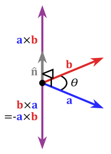
The cross product a × b is defined as a vector c that is perpendicular (orthogonal) to both a and b, with a direction given by the right-hand rule and a magnitude equal to the area of the parallelogram that the vectors span.
The cross product is defined by the formula[3][4]

- where θ is the angle between a and b in the plane containing them (hence, it is between 0° and 180°), ‖a‖ and ‖b‖ are the magnitudes of vectors a and b, and n is a unit vector perpendicular to the plane containing a and bin the direction given by the right-hand rule (illustrated). If the vectors a and b are parallel (i.e., the angle θ between them is either 0° or 180°), by the above formula, the cross product of a and b is the zero vector 0.
By convention, the direction of the vector n is given by the right-hand rule, where one simply points the forefinger of the right hand in the direction of a and the middle finger in the direction of b. Then, the vector n is coming out of the thumb (see the picture on the right). Using this rule implies that the cross product is anti-commutative, i.e., b × a = −(a × b). By pointing the forefinger toward b first, and then pointing the middle finger toward a, the thumb will be forced in the opposite direction, reversing the sign of the product vector.
Using the cross product requires the handedness of the coordinate system to be taken into account (as explicit in the definition above). If a left-handed coordinate system is used, the direction of the vector n is given by the left-hand rule and points in the opposite direction.
This, however, creates a problem because transforming from one arbitrary reference system to another (e.g., a mirror image transformation from a right-handed to a left-handed coordinate system), should not change the direction of n. The problem is clarified by realizing that the cross product of two vectors is not a (true) vector, but rather a pseudovector. See cross product and handedness for more detail.
Names

According to Sarrus’s rule, the determinant of a 3×3 matrix involves multiplications between matrix elements identified by crossed diagonals
In 1881, Josiah Willard Gibbs, and independently Oliver Heaviside, introduced both the dot product and the cross product using a period (a . b) and an “x” (a x b), respectively, to denote them.[5]
In 1877, to emphasize the fact that the result of a dot product is a scalar while the result of a cross product is a vector, William Kingdon Clifford coined the alternative namesscalar product and vector product for the two operations.[5] These alternative names are still widely used in the literature.
Both the cross notation (a × b) and the name cross product were possibly inspired by the fact that each scalar component of a × b is computed by multiplying non-corresponding components of a and b. Conversely, a dot product a ⋅ b involves multiplications between corresponding components of a and b. As explained below, the cross product can be expressed in the form of a determinant of a special 3 × 3 matrix. According to Sarrus’s rule, this involves multiplications between matrix elements identified by crossed diagonals.
之後,將會 …… 耶☆


 三個坐標來描述;或者在
 三個坐標描述。描述系統的坐標可以自由的選取,但獨立坐標的個數總是一定的,即系統的自由度。一般而言,
 個質點組成的力學系統由
  個坐標來描述。但力學系統中常常存在著各種
 個
個


![\displaystyle {\begin{aligned}\ [1,3,-5]\cdot [4,-2,-1]&=(1)(4)+(3)(-2)+(-5)(-1)\\&=4-6+5\\&=3\end{aligned}}](http://www.freesandal.org/wp-content/ql-cache/quicklatex.com-318ca23e7041466f909fe49b86988388_l3.png "Rendered by QuickLaTeX.com")
 .
. means the

 .
. . The dot product of two Euclidean vectors a and b is defined by


![\displaystyle \mathbf {K} =\left[{\begin{array}{ccc}0&-k_{z}&k_{y}\\k_{z}&0&-k_{x}\\-k_{y}&k_{x}&0\end{array}}\right]\,,](http://www.freesandal.org/wp-content/ql-cache/quicklatex.com-6dd7dd45d725e0b0b4247e553d45492f_l3.png "Rendered by QuickLaTeX.com")


 (3) = ℝ3


 .
.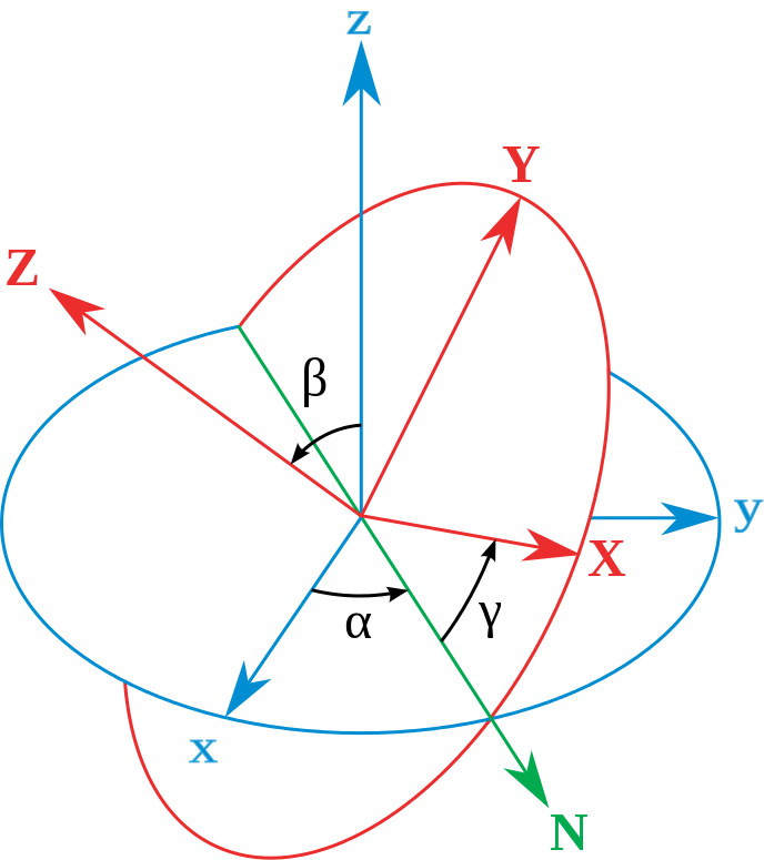
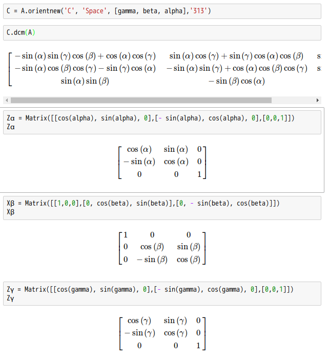
![\displaystyle [\mathbf {R} ]](http://www.freesandal.org/wp-content/ql-cache/quicklatex.com-3409ff25d6f5cdd4fa1befd19bd3df62_l3.png "Rendered by QuickLaTeX.com") 是由三個基本旋轉矩陣合成的:
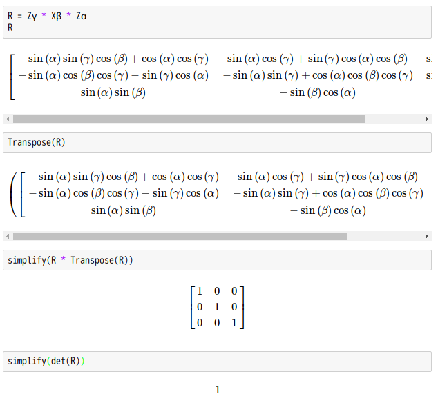
是由三個基本旋轉矩陣合成的:![\displaystyle [\mathbf {R} ]={\begin{bmatrix}\cos \gamma &\sin \gamma &0\\-\sin \gamma &\cos \gamma &0\\0&0&1\end{bmatrix}}{\begin{bmatrix}1&0&0\\0&\cos \beta &\sin \beta \\0&-\sin \beta &\cos \beta \end{bmatrix}}{\begin{bmatrix}\cos \alpha &\sin \alpha &0\\-\sin \alpha &\cos \alpha &0\\0&0&1\end{bmatrix}}](http://www.freesandal.org/wp-content/ql-cache/quicklatex.com-f9b05d1323eada3a1326bcdfb0d8ed30_l3.png "Rendered by QuickLaTeX.com")
![\displaystyle [\mathbf {R} ]={\begin{bmatrix}\cos \alpha \cos \gamma -\cos \beta \sin \alpha \sin \gamma &\sin \alpha \cos \gamma +\cos \beta \cos \alpha \sin \gamma &\sin \beta \sin \gamma \\-\cos \alpha \sin \gamma -\cos \beta \sin \alpha \cos \gamma &-\sin \alpha \sin \gamma +\cos \beta \cos \alpha \cos \gamma &\sin \beta \cos \gamma \\\sin \beta \sin \alpha &-\sin \beta \cos \alpha &\cos \beta \end{bmatrix}}](http://www.freesandal.org/wp-content/ql-cache/quicklatex.com-1aea915f7324ab40e84bbfdf9cfcda66_l3.png "Rendered by QuickLaTeX.com")
![\displaystyle [\mathbf {R} ]^{-1}={\begin{bmatrix}\cos \alpha \cos \gamma -\cos \beta \sin \alpha \sin \gamma &-\cos \alpha \sin \gamma -\cos \beta \sin \alpha \cos \gamma &\sin \beta \sin \alpha \\\sin \alpha \cos \gamma +\cos \beta \cos \alpha \sin \gamma &-\sin \alpha \sin \gamma +\cos \beta \cos \alpha \cos \gamma &-\sin \beta \cos \alpha \\\sin \beta \sin \gamma &\sin \beta \cos \gamma &\cos \beta \end{bmatrix}}](http://www.freesandal.org/wp-content/ql-cache/quicklatex.com-17072c040bc89d6b6f9ac81cca10c3cb_l3.png "Rendered by QuickLaTeX.com")
 ,在 xy z與 XYZ坐標系統的坐標分別為
  與
與  。定義角算符
  為繞著Z-軸旋轉
  。
。 ,
, ,
, 。
。 ,在 xyz 與 XYZ 坐標系統的坐標分別為
  與
與  。定義角算符
  為繞著z-軸旋轉
  。
。 ,
, ,
, 。
。 那麼,
那麼, 。
。 。
。 ,
, ,
, 。
。 ,
, 。
。