Michael Nielsen 先生此段文字是本章的重點，他先從

The Hadamard product, $s \odot t$

The backpropagation algorithm is based on common linear algebraic operations – things like vector addition, multiplying a vector by a matrix, and so on. But one of the operations is a little less commonly used. In particular, suppose $s$ and $t$ are two vectors of the same dimension. Then we use $s \odot t$ $s ⊙ t$ to denote the elementwise product of the two vectors. Thus the components of $s \odot t$ $s ⊙ t$ are just $(s \odot t)_j = s_j t_j$ $(s ⊙ t)_{j} = s_{j} t_{j}$ . As an example,

\left[\begin{array}{c} 1 \\ 2 \end{array}\right] \odot \left[\begin{array}{c} 3 \\ 4\end{array} \right] = \left[ \begin{array}{c} 1 * 3 \\ 2 * 4 \end{array} \right] = \left[ \begin{array}{c} 3 \\ 8 \end{array} \right]. \ \ \ \ (28)

This kind of elementwise multiplication is sometimes called the Hadamard product or Schur product. We’ll refer to it as the Hadamard product. Good matrix libraries usually provide fast implementations of the Hadamard product, and that comes in handy when implementing backpropagation.

───

講起，是希望藉著『記號法』，方便讀者理解『反向傳播算法』的內容。這個稱作 Hadamard product 之『對應元素乘法』

Hadamard product (matrices)

In mathematics, the Hadamard product (also known as the Schur product^[1] or the entrywise product^[2]) is a binary operation that takes two matrices of the same dimensions, and produces another matrix where each element ij is the product of elements ij of the original two matrices. It should not be confused with the more common matrix product. It is attributed to, and named after, either French mathematician Jacques Hadamard, or German mathematician Issai Schur.

The Hadamard product is associative and distributive, and unlike the matrix product it is also commutative.

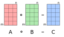
The Hadamard product operates on identically-shaped matrices and produces a third matrix of the same dimensions.

Definition

For two matrices, $A, B$ , of the same dimension, $m \times n$ the Hadamard product, $A \circ B$ , is a matrix, of the same dimension as the operands, with elements given by

(A \circ B)_{i,j} = (A)_{i,j} \cdot (B)_{i,j}

For matrices of different dimensions ( $m \times n$ and $p \times q$ , where $m \not= p$ or $n \not= q$ or both) the Hadamard product is undefined.

Example

For example, the Hadamard product for a 3×3 matrix A with a 3×3 matrix B is:

\left(\begin{array}{ccc} \mathrm{a}_{11} & \mathrm{a}_{12} & \mathrm{a}_{13}\\ \mathrm{a}_{21} & \mathrm{a}_{22} & \mathrm{a}_{23}\\ \mathrm{a}_{31} & \mathrm{a}_{32} & \mathrm{a}_{33} \end{array}\right) \circ \left(\begin{array}{ccc} \mathrm{b}_{11} & \mathrm{b}_{12} & \mathrm{b}_{13}\\ \mathrm{b}_{21} & \mathrm{b}_{22} & \mathrm{b}_{23}\\ \mathrm{b}_{31} & \mathrm{b}_{32} & \mathrm{b}_{33} \end{array}\right) = \left(\begin{array}{ccc} \mathrm{a}_{11}\, \mathrm{b}_{11} & \mathrm{a}_{12}\, \mathrm{b}_{12} & \mathrm{a}_{13}\, \mathrm{b}_{13}\\ \mathrm{a}_{21}\, \mathrm{b}_{21} & \mathrm{a}_{22}\, \mathrm{b}_{22} & \mathrm{a}_{23}\, \mathrm{b}_{23}\\ \mathrm{a}_{31}\, \mathrm{b}_{31} & \mathrm{a}_{32}\, \mathrm{b}_{32} & \mathrm{a}_{33}\, \mathrm{b}_{33} \end{array}\right)

───

明晰易解，大概無需畫蛇添足的吧！然而接下來的『妖怪說』︰

The four fundamental equations behind backpropagation

Backpropagation is about understanding how changing the weights and biases in a network changes the cost function. Ultimately, this means computing the partial derivatives $\partial C / \partial w^l_{jk}$ $\partial C / \partial w_{j k}^{l}$ and $\partial C / \partial b^l_j$ $\partial C / \partial b_{j}^{l}$ . But to compute those, we first introduce an intermediate quantity, $\delta^l_j$ $δ_{j}^{l}$ , which we call the error in the $j^{\rm th}$ $j^{t h}$ neuron in the $l^{\rm th}$ $l^{t h}$ layer. Backpropagation will give us a procedure to compute the error $\delta^l_j$ $δ_{j}^{l}$ , and then will relate $\delta^l_j$ $δ_{j}^{l}$ to $\partial C / \partial w^l_{jk}$ $\partial C / \partial w_{j k}^{l}$ and $\partial C / \partial b^l_j$ $\partial C / \partial b_{j}^{l}$ .

To understand how the error is defined, imagine there is a demon in our neural network:

The demon sits at the $j^{\rm th}$

j^{t h}

neuron in layer $l$

l

. As the input to the neuron comes in, the demon messes with the neuron’s operation. It adds a little change $\Delta z^l_j$

Δ z_{j}^{l}

to the neuron’s weighted input, so that instead of outputting $\sigma(z^l_j)$

σ (z_{j}^{l})

, the neuron instead outputs $\sigma(z^l_j+\Delta z^l_j)$

σ (z_{j}^{l} + Δ z_{j}^{l})

. This change propagates through later layers in the network, finally causing the overall cost to change by an amount $\frac{\partial C}{\partial z^l_j} \Delta z^l_j$

\frac{\partial C}{\partial z_{j}^{l}} Δ z_{j}^{l}

Now, this demon is a good demon, and is trying to help you improve the cost, i.e., they’re trying to find a $\Delta z^l_j$ $Δ z_{j}^{l}$ which makes the cost smaller. Suppose $\frac{\partial C}{\partial z^l_j}$ $\frac{\partial C}{\partial z_{j}^{l}}$ has a large value (either positive or negative). Then the demon can lower the cost quite a bit by choosing $\Delta z^l_j$ $Δ z_{j}^{l}$ to have the opposite sign to $\frac{\partial C}{\partial z^l_j}$ $\frac{\partial C}{\partial z_{j}^{l}}$ . By contrast, if $\frac{\partial C}{\partial z^l_j}$ $\frac{\partial C}{\partial z_{j}^{l}}$ is close to zero, then the demon can’t improve the cost much at all by perturbing the weighted input $z^l_j$ $z_{j}^{l}$ . So far as the demon can tell, the neuron is already pretty near optimal*

*This is only the case for small changes $\Delta z^l_j$ $Δ z_{j}^{l}$ , of course. We’ll assume that the demon is constrained to make such small changes..

And so there’s a heuristic sense in which $\frac{\partial C}{\partial z^l_j}$ $\frac{\partial C}{\partial z_{j}^{l}}$ is a measure of the error in the neuron.

Motivated by this story, we define the error $\delta^l_j$ $δ_{j}^{l}$ of neuron $j$ $j$ in layer $l$ $l$ by

\delta^l_j \equiv \frac{\partial C}{\partial z^l_j}. \ \ \ \ (29)

As per our usual conventions, we use $\delta^l$ $δ^{l}$ to denote the vector of errors associated with layer $l$ $l$ . Backpropagation will give us a way of computing $\delta^l$ $δ^{l}$ for every layer, and then relating those errors to the quantities of real interest, $\partial C / \partial w^l_{jk}$ $\partial C / \partial w_{j k}^{l}$ and $\partial C / \partial b^l_j$ $\partial C / \partial b_{j}^{l}$ .

You might wonder why the demon is changing the weighted input $z^l_j$ $z_{j}^{l}$ . Surely it’d be more natural to imagine the demon changing the output activation $a^l_j$ $a_{j}^{l}$ , with the result that we’d be using $\frac{\partial C}{\partial a^l_j}$ $\frac{\partial C}{\partial a_{j}^{l}}$ as our measure of error. In fact, if you do this things work out quite similarly to the discussion below. But it turns out to make the presentation of backpropagation a little more algebraically complicated. So we’ll stick with $\delta^l_j = \frac{\partial C}{\partial z^l_j}$ $δ_{j}^{l} = \frac{\partial C}{\partial z_{j}^{l}}$ as our measure of error*

*In classification problems like MNIST the term “error” is sometimes used to mean the classification failure rate. E.g., if the neural net correctly classifies 96.0 percent of the digits, then the error is 4.0 percent. Obviously, this has quite a different meaning from our $\delta$ $δ$ vectors. In practice, you shouldn’t have trouble telling which meaning is intended in any given usage..

───

確須仔細斟詳，方可確實明白，達成為我所用之目的。或因 Michael Nielsen 先生不能假設讀者知道『矩陣』、『向量』以及『無窮小』之『萊布尼茲記號法』︰

Leibniz’s notation

In calculus, Leibniz’s notation, named in honor of the 17th-century German philosopher and mathematician Gottfried Wilhelm Leibniz, uses the symbols $dx$ and $dy$ to represent infinitely small (or infinitesimal) increments of $x$ and $y$ , respectively, just as $Δ x$ and $Δ y$ represent finite increments of $x$ and $y$ , respectively.^[1]

Consider $y$ as a function of a variable $x$ , or $y$ = $f (x)$ . If this is the case, then the derivative of $y$ with respect to $x$ , which later came to be viewed as the limit

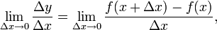
\lim_{\Delta x\rightarrow 0}\frac{\Delta y}{\Delta x} = \lim_{\Delta x\rightarrow 0}\frac{f(x + \Delta x)-f(x)}{\Delta x},

was, according to Leibniz, the quotient of an infinitesimal increment of $y$ by an infinitesimal increment of $x$ , or

\frac{dy}{dx}=f'(x),

where the right hand side is Joseph-Louis Lagrange’s notation for the derivative of $f$ at $x$ . From the point of view of modern infinitesimal theory, $Δ x$ is an infinitesimal $x$ -increment, $Δ y$ is the corresponding $y$ -increment, and the derivative is the standard part of the infinitesimal ratio:

f'(x)={\rm st}\Bigg( \frac{\Delta y}{\Delta x} \Bigg)

Then one sets $dx=\Delta x$ , $dy = f'(x) dx\,$ , so that by definition, $f'(x)\,$ is the ratio of dy by dx.

Similarly, although mathematicians sometimes now view an integral

\int f(x)\,dx

as a limit

\lim_{\Delta x\rightarrow 0}\sum_{i} f(x_i)\,\Delta x,

where $Δ x$ is an interval containing $x i$ , Leibniz viewed it as the sum (the integral sign denoting summation) of infinitely many infinitesimal quantities $f (x) dx$ . From the modern viewpoint, it is more correct to view the integral as the standard part of such an infinite sum.

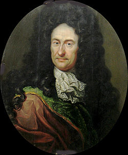
250px-Gottfried_Wilhelm_Leibniz_c1700

Gottfried Wilhelm von Leibniz (1646 – 1716), German philosopher, mathematician, and namesake of this widely used mathematical notation in calculus.

───

於是方用迂迴的方式來說。如果回顧相干函式關係︰

$C = C({\vec a}^L)$

${\vec a}^L = \sigma ({\vec z}^L)$

$\begin{array}{rcl} (3) & σ (z) \equiv \frac{1}{1 + e^{- z}} . \end{array}$

${\vec z}^{\ l} \ \equiv \ W^{\ l} \ {\vec a}^{\ l-1} \ + \ {\vec b}^{\ l}$

也許會發現之所以選擇 $C = C({\vec z}^L)$ 自然而然順理成章。若是通熟『鏈式法則』

Chain rule

In calculus, the chain rule is a formula for computing the derivative of the composition of two or more functions. That is, if f and g are functions, then the chain rule expresses the derivative of their composition f ∘ g (the function which maps x to f(g(x)) in terms of the derivatives of f and g and the product of functions as follows:

(f\circ g)'=(f'\circ g)\cdot g'.

This can be written more explicitly in terms of the variable. Let F = f ∘ g, or equivalently, F(x) = f(g(x)) for all x. Then one can also write

F'(x) = f'(g(x)) g'(x).

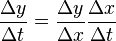
The chain rule may be written, in Leibniz’s notation, in the following way. We consider z to be a function of the variable y, which is itself a function of x (y and z are therefore dependent variables), and so, z becomes a function of x as well:

\frac{dz}{dx} = \frac{dz}{dy} \cdot \frac{dy}{dx}.

In integration, the counterpart to the chain rule is the substitution rule.

……

Proof via infinitesimals

If $y=f(x)$ and $x=g(t)$ then choosing infinitesimal $\Delta t\not=0$ we compute the corresponding 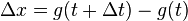$\Delta x=g(t+\Delta t)-g(t)$ and then the corresponding $\Delta y=f(x+\Delta x)-f(x)$ , so that

\frac{\Delta y}{\Delta t}=\frac{\Delta y}{\Delta x} \frac{\Delta x}{\Delta t}

and applying the standard part we obtain

\frac{d y}{d t}=\frac{d y}{d x} \frac{dx}{dt}

which is the chain rule.

───

該文本之內容會是天經地義無可疑議矣？？！！由於『微積分』是閱讀科技著作和文獻之『必修課』與『先修課』，它的深入理解以及直覺掌握，將有莫大價值，故而作者曾假《觀水》一文中京房之『上飛下飛』十六變之法，寫了

《【Sonic π】電路學之補充《四》無窮小算術‧…》一系列文本，期望能助益於萬一也！！？？

最後補以『觀察點』之選擇往往會造成不同的『難易度』！！！

具體數學：計算機科學之基石

An ant starts to crawl along a taut rubber rope 1 km long at a speed of 1 cm per second (relative to the rubber it is crawling on). At the same time, the rope starts to stretch uniformly by 1 km per second, so that after 1 second it is 2 km long, after 2 seconds it is 3 km long, etc. Will the ant ever reach the end of the rope?

在『具體數學』這本書中提到了另一個『違反直覺』的例子 ── 橡膠繩上的螞蟻 ──，一隻螞蟻以每秒鐘一公分的速度，在一根長一公里拉緊了的橡膠繩上爬行【螞蟻的爬行速度相對橡膠繩】，就在螞蟻爬行的同時，橡膠繩也以每秒一公里的速度伸長，也就是說一秒後，它有兩公里長，兩秒後有三公里長等等。試問螞蟻果真到的了繩子之另一端的嗎？

假設 $t$ 時刻時，螞蟻在 $x(t), x_0 = x(0)$ 的『位置』，以 $\alpha$ 的速度朝另一端爬行，同時橡膠繩用 $v$ 的速度同向均勻伸長，因此橡膠繩上的某點 $X$ 的伸長速度將是 $\frac{X}{c + v t} v$ ，此處 $c$ 就是橡膠繩的『原長』，由於起點是『固定』不動的，因此繩上各點的速度與『端點的速度』 $v = \frac{c + v t}{c + v t} v$ 成比例，於是對於一個靜止的觀察者而言，螞蟻的速度將是

$\frac{dx(t)}{dt} = x'(t) = \alpha+\frac{x(t)}{c+vt} v$

。如果我們設想要是橡膠繩並不與時伸展，那麼這隻螞蟻是一定到的了彼端，假使一個相對於繩子靜止的觀察者將看到什麼現象的呢？或許他將用 $\Phi (t) = \frac{x(t)}{c + v t}$ 來描述這隻螞蟻的行進的吧！它從 $t=0, \Phi(0) = 0$ 開始爬行，它將會在 $t=T, \Phi(T)=1$ 時刻到達了另一端。由於

$\frac{d\Phi}{dt} = \frac{d}{dt} \left[ {(c + v t)}^{-1} \cdot x(t) \right]$
$= {(c + v t)}^{-1} \cdot \frac{dx(t)}{dt} - {(c + v t)}^{-2} \cdot v x(t)$
$= {(c + v t)}^{-1} \cdot \left[ \alpha + {(c + v t)}^{-1} \cdot v x(t) \right] - {(c + v t)}^{-2} \cdot v x(t)$
$= \frac{\alpha}{c + v t}$ ，因此我們就可以得到

$\Phi(t)=\int{\frac{\alpha}{c+vt}\,dt}=\frac{\alpha}{v}\log(c+vt)+\kappa$

此處 $\kappa$ 積分常數。從 $\Phi(0)=0$ ，可以得到 $\kappa=-\frac{\alpha}{v}\log{c}$ ，所以 $\Phi(t)=\frac{\alpha}{v}\log{\left(\frac{c+vt}{c}\right)}$ 。再從 $\Phi(T)=1$ ，就得到了 $T=\frac{c}{v}\left(e^{v/\alpha}-1\right)$ 。

假使將 $c = 1 km, v = 1 km/sec, \alpha = 1 cm/sec$ 代入後，求得 $T=(e^{100,000}-1) \ \mathrm{s}\ \approx2.8\times10^{43,429}\,\mathrm{s}$ ，這隻小螞蟻果真到的了彼端，雖然它得經過千千萬萬個三千大劫的吧！！

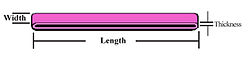
那麼為什麼︰某點 $X$ 的伸長速度會是 $\frac{X}{c + v t} v$ 的呢？假使考慮一根『有刻度』 $p_i, i = 0 \cdots n$ 的尺，它的一端固定，另一端向外延伸，這樣每個『刻度點』也都相對的向外伸長 ${\delta}_i$ ，於是『固定端』 ${\delta}_0 =0$ ，『第一個刻度』在 $p_1 + {\delta}_1$ 的位置，『第二個刻度』在 $p_2 + {\delta}_1+ {\delta}_2$ 的位置，這樣『第 $k$ 個刻度』將在 $p_k + \sum \limits_{j=1}^{j=k} {\delta}_j$ 的位置。假設『橡膠繩』的『彈性』是『均勻』的，這樣所有的 ${\delta}_i = \delta x$ 都相等，因此 $p_k + \sum \limits_{j=1}^{j=k} {\delta}_j = p_k + k \delta x$ ，如此當『另一端』用『定速』 $v$ 移動時，此時 $n \delta x = v \delta t$ ，於是『第 $k$ 個刻度』就用 $\frac{k}{n} v$ 的速度在移動的啊！

過去有人曾經想像過一種情況︰如果說宇宙中的一切，在夜間會突然的『變大』或者『縮小』，那麼我們能夠『發現』的嗎？假使從『量測』的觀點來看，如果度量用的『尺』 $l_{\lambda} = \lambda l_0$ 隨著時間改變，『被度量事物』的『大小』 $S_0$ 也『協同』的跟隨著變化 $S(t) = \lambda \cdot S_0$ ，這樣在那個『宇宙』裡面 $\frac{S(t)}{l_{\lambda} } = \frac{S_0}{l_0}$ ，也就是講『測量』沒有辦法『知道』到底『有沒有』發生過這件事的啊！！然而這卻更進一步引發了『自然定律』到底是否會在『度量單位』的改變下，而有所不同的呢？？