如何深入了解一個重要的定律︰
大數定律
在數學與統計學中,大數定律又稱大數法則、大數律,是描述相當多次數重複實驗的結果的定律。根據這個定律知道,樣本數量越多 ,則其平均就越趨近期望值。
大數定律很重要,因為它「保證」了一些隨機事件的均值的長期穩定性。人們發現,在重複試驗中,隨著試驗次數的增加,事件發生的頻率趨於一個穩定值;人們同時也發現,在對物理量的測量實踐中,測定值的算術平均也具有穩定性。比如,我們向上拋一枚硬幣 ,硬幣落下後哪一面朝上本來是偶然的,但當我們上拋硬幣的次數足夠多後,達到上萬次甚至幾十萬幾百萬次以後,我們就會發現,硬幣每一面向上的次數約占總次數的二分之一。偶然之中包含著必然。
切比雪夫定理的一個特殊情況、辛欽定理和伯努利大數定律都概括了這一現象,都稱為大數定律。
表現形式
大數定律主要有兩種表現形式:弱大數定律和強大數定律。定律的兩種形式都肯定無疑地表明,樣本均值

收斂於真值

其中 X1, X2, … 是獨立同分布的,期望值 E(X1) = E(X2) = …= µ 的,勒貝格可積的隨機變量構成的無窮序列。Xj 的勒貝格可積性意味著期望值 E(Xj) 存在且有限。
方差 Var(X1) = Var(X2) = … = σ2 < ∞ 有限的假設是非必要的。很大或者無窮大的方差會使其收斂得緩慢一些,但大數定律仍然成立。通常採用這個假設來使證明更加簡潔。
強和弱之間的差別在所斷言的收斂的方式。對於這些方式的解釋,參見隨機變量的收斂。
有時候不只要知道它的推導過程︰
Proof of the weak law
Given X1, X2, … an infinite sequence of i.i.d. random variables with finite expected value E(X1) = E(X2) = … = µ < ∞, we are interested in the convergence of the sample average

The weak law of large numbers states:
Theorem:  |
|
(law. 2) |
Proof using Chebyshev’s inequality
This proof uses the assumption of finite variance 


The common mean μ of the sequence is the mean of the sample average:

Using Chebyshev’s inequality on 

This may be used to obtain the following:

As n approaches infinity, the expression approaches 1. And by definition of convergence in probability, we have obtained
還要能知道有沒有反例︰
柯西分布
柯西分布也叫作柯西-勞侖茲分布,它是以奧古斯丁·路易·柯西與亨德里克·勞侖茲名字命名的連續機率分布,其機率密度函數為
![f(x; x_0,\gamma) = \frac{1}{\pi\gamma \left[1 + \left(\frac{x-x_0}{\gamma}\right)^2\right]} \!](https://wikimedia.org/api/rest_v1/media/math/render/svg/4a27e55208fcb481a2a5efcde57564590840870e)
![= { 1 \over \pi } \left[ { \gamma \over (x - x_0)^2 + \gamma^2 } \right] \!](https://wikimedia.org/api/rest_v1/media/math/render/svg/fd9b7edf06364f64f8dcfccc4d5bbccba62abacf)
其中x0是定義分布峰值位置的位置參數,γ是最大值一半處的一半寬度的尺度參數。
作為機率分布,通常叫作柯西分布,物理學家也將之稱為勞侖茲分布或者Breit-Wigner分布。在物理學中的重要性很大一部分歸因於它是描述受迫共振的微分方程式的解。在光譜學中,它描述了被共振或者其它機制加寬的譜線形狀。在下面的部分將使用柯西分布這個統計學術語。
x0 = 0且γ = 1的特例稱為標準柯西分布,其機率密度函數為

特性
其累積分布函數為:

柯西分布的逆累積分布函數為

柯西分布的平均值、變異數或者矩都沒有定義,它的眾數與中值有定義都等於 x0。
取 X 表示柯西分布隨機變量,柯西分布的特性函數表示為:

如果 U 與 V 是期望值為 0、變異數為 1 的兩個獨立常態分布隨機變量的話,那麼比值 U/V 為柯西分布。
標準柯西分布是學生t-分布自由度為1的特殊情況。
柯西分布是穩定分布:如果 

如果 X1, …, Xn 是分別符合柯西分布的相互獨立同分布隨機變量,那麼算術平均數(X1 + … + Xn)/n 有同樣的柯西分布。為了證明這一點,我們來計算採樣平均的特性函數:

其中, 
洛侖茲線性分布更適合於那種比較扁、寬的曲線 高斯線性分布則適合較高、較窄的曲線 當然,如果是比較居中的情況,兩者都可以。 很多情況下,採用的是兩者各占一定比例的做法。如勞侖次占60%,高斯占40%.
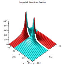
Lorentzian function Imaginary part Maple complex 3D plot
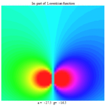
Imaginary plot of Lorentzian function (Maple animation)
清楚明白違背的理由︰
Explanation of undefined moments
Mean
If a probability distribution has a density function f(x), then the mean is

The question is now whether this is the same thing as

for an arbitrary real number a.
If at most one of the two terms in (2) is infinite, then (1) is the same as (2). But in the case of the Cauchy distribution, both the positive and negative terms of (2) are infinite. Hence (1) is undefined.[12]
Note that the Cauchy principal value of the Cauchy distribution is:

which is zero, while:

is not zero, as can be seen easily by computing the integral.
Various results in probability theory about expected values, such as the strong law of large numbers, will not work in such cases.[12]
Higher moments
The Cauchy distribution does not have finite moments of any order. Some of the higher raw moments do exist and have a value of infinity, for example the raw second moment:
![{\begin{aligned}{\mathrm {E}}[X^{2}]&\propto \int _{{-\infty }}^{\infty }{\frac {x^{2}}{1+x^{2}}}\,dx=\int _{{-\infty }}^{\infty }1-{\frac {1}{1+x^{2}}}\,dx\\[8pt]&=\int _{{-\infty }}^{\infty }dx-\int _{{-\infty }}^{\infty }{\frac {1}{1+x^{2}}}\,dx=\int _{{-\infty }}^{\infty }dx-\pi =\infty .\end{aligned}}](https://wikimedia.org/api/rest_v1/media/math/render/svg/9330fe0651a9eb2248e439214a55d11949c8cdc0)
By re-arranging the formula, one can see that the second moment is essentially the infinite integral of a constant (here 1). Higher even-powered raw moments will also evaluate to infinity. Odd-powered raw moments, however, are undefined, which is distinctly different from existing with the value of infinity. The odd-powered raw moments are undefined because their values are essentially equivalent to 
The results for higher moments follow from Hölder’s inequality, which implies that higher moments (or halves of moments) diverge if lower ones do.
且試著追溯它的歷史︰
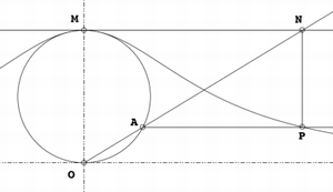
箕舌線
箕舌線是平面曲線的一種,也被稱為阿涅西的女巫(英語:The Witch of Agnesi)[1][2][3]。
給定一個圓和圓上的一點O。對於圓上的任何其它點A,作割線OA。設M是O的對稱點。OA與M的切線相交於N。過N且與OM平行的直線,與過A且與OM垂直的直線相交於P。則P的軌跡就是箕舌線。
箕舌線有一條漸近線,它是上述給定圓過O點的切線。
方程
設O是原點,M在正的y軸上。假設圓的半徑是a。
則曲線的方程為 
注意如果a=1/2,則曲線化為最簡單的形式:

如果 

如果

箕舌線
歷史
皮埃爾·德·費馬曾在1630年研究這條曲線。1703年時格蘭迪提出了建構這條曲線的方法。1718年時格蘭迪建議將這條曲線命名為versoria,意思是張帆的繩子,並將這條曲線的義大利文名稱命名為versiera[4]
1748年時瑪利亞·阿涅西出版了著名的著作《Instituzioni analitiche ad uso della gioventù italiana》,其中箕舌線仍沿用格蘭迪取的名稱versiera[4],一恰好當時的義大利文Aversiera/Versiera是衍生自拉丁文的Adversarius,是魔鬼的一個稱呼「與神為敵的」,和女巫是同義詞[5]。也許因為這個原因,劍橋教授 約翰·科爾森就誤譯了這條曲線。許多近代有關阿涅西及此曲線的著作對於誤譯的原因有些不同的猜測[6][7][8]斯特洛伊克認為:
versiera這個字是衍生自拉丁文的vertere,但後者也是義大利文avversiera(女魔鬼)的縮寫。英格蘭有些聰敏者將之翻譯成女巫(英語:witch),而這好笑的雙關語仍存於多數的英文教材裡。在費馬的著作(Oeuvres, I, 279-280; III, 233-234)就已經出現這條曲線,其名稱versiera是格蘭迪取的,在牛頓的曲線分類中,它是第63類……第一個使用女巫來描述這條曲線的可能是威廉森在1875年的《Integral calculus》中首次使用[9]
另一方面,史蒂芬·史蒂格勒認為是格蘭迪自已在玩文字遊戲[10]。
應用
箕舌線除了其理論的性質外.也常出現在現實生活中.不過這次應用是在20世紀末期及21世紀才有足夠的了解。在為一些物體現象建立數學模型時,會出現箕舌線[11]。 此方程式近似光線及X光的譜線分布,也是共振電路中的能量耗散量。
光滑小山嶽的截面也類似箕舌線。在數學建模中已用箕舌線作為一種流場的障礙物[12][13]。
確定論理之條件︰
馬爾可夫不等式
在機率論中,馬爾可夫不等式給出了隨機變量的函數大於等於某正數的機率的上界。雖然它以俄國數學家安德雷·馬爾可夫命名,但該不等式曾出現在一些更早的文獻中,其中包括馬爾可夫的老師–巴夫尼提·列波維奇·切比雪夫。
馬爾可夫不等式把機率關聯到數學期望,給出了隨機變量的累積分布函數一個寬泛但仍有用的界。
馬爾可夫不等式的一個應用是,不超過1/5的人口會有超過5倍於人均收入的收入。
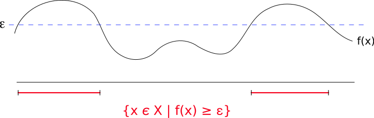
馬爾可夫不等式提供了 


表達式
X為一非負隨機變量,則

若用測度領域的術語來表示,馬爾可夫不等式可表示為若(X, Σ, μ)是一個測度空間,ƒ為可測的擴展實數的函數,且 

對於單調增加函數的擴展版本
若φ是定義在非負實數上的單調增加函數,且其值非負,X是一個隨機變量,a ≥ 0,且φ(a) > 0,則

用來推論切比雪夫不等式
切比雪夫不等式使用變異數來作為一隨機變數超過平均值機率的上限,可以用下式表示:

對任意a>0,Var(X)為X的變異數,定義如下:
![\operatorname {Var}(X)=\operatorname {E}[(X-\operatorname {E}(X))^{2}].](https://wikimedia.org/api/rest_v1/media/math/render/svg/71c7a116967cab98cb1eb56e626497e77ce354a2)
若以馬爾可夫不等式為基礎,切比雪夫不等式可視為考慮以下隨機變數

根據馬爾可夫不等式,可得到以下的結果
