乍看之下, Michael Nielsen 先生之此段文本︰
The two assumptions we need about the cost function
The goal of backpropagation is to compute the partial derivatives  and
and  of the cost function
  with respect to any weight w or bias b in the network. For backpropagation to work we need to make two main assumptions about the form of the cost function. Before stating those assumptions, though, it’s useful to have an example cost function in mind. We’ll use the quadratic cost function from last chapter (c.f. Equation (6)). In the notation of the last section, the quadratic cost has the form

where:  is the total number of training examples; the sum is over individual training examples,
  ;
;  is the corresponding desired output;
  denotes the number of layers in the network; and
  is the vector of activations output from the network when is input.
Okay, so what assumptions do we need to make about our cost function, , in order that backpropagation can be applied? The first assumption we need is that the cost function can be written as an average  over cost functions
  for individual training examples, . This is the case for the quadratic cost function, where the cost for a single training example is
  . This assumption will also hold true for all the other cost functions we’ll meet in this book.
The reason we need this assumption is because what backpropagation actually lets us do is compute the partial derivatives  and
and  for a single training example. We then recover and by averaging over training examples. In fact, with this assumption in mind, we’ll suppose the training example has been fixed, and drop the subscript, writing the cost as . We’ll eventually put the x back in, but for now it’s a notational nuisance that is better left implicit.
The second assumption we make about the cost is that it can be written as a function of the outputs from the neural network:


and thus is a function of the output activations. Of course, this cost function also depends on the desired output  , and you may wonder why we’re not regarding the cost also as a function of . Remember, though, that the input training example is fixed, and so the output is also a fixed parameter. In particular, it’s not something we can modify by changing the weights and biases in any way, i.e., it’s not something which the neural network learns. And so it makes sense to regard as a function of the output activations
  alone, with merely a parameter that helps define that function.
───
簡單易明!其實梳理實在費事?首先我們將式子 (26) 改寫如下

。
假使從『黑箱』角度來看,如果『輸入』是  ,神經網絡之『目標輸出』是
  ,當下『訓練』之『輸出』是
  。如是對『訓練樣本』 而言,如將此神經網絡的『目標誤差』定義為
  。那麼『函式』 就是所有之 個『訓練樣本』的『平均』『目標誤差』。若是仔細審查
  的定義,將可發現它就是兩向量之『歐式距離』之半,其實是個『純量』。而且所謂的『訓練樣本』 以及『目標輸出』 事實上都只是『參數』︰
Parameter
A parameter (from the Ancient Greek παρά, “para”, meaning “beside, subsidiary” and μέτρον, “metron”, meaning “measure”), in its common meaning, is a characteristic, feature, or measurable factor that can help in defining a particular system. A parameter is an important element to consider in evaluation or comprehension of an event, project, or situation. Parameter has more specific interpretations in mathematics, logic, linguistics, environmental science, and other disciplines.[1]
Mathematical functions
Mathematical functions have one or more arguments that are designated in the definition by variables. A function definition can also contain parameters, but unlike variables, parameters are not listed among the arguments that the function takes. When parameters are present, the definition actually defines a whole family of functions, one for every valid set of values of the parameters. For instance, one could define a general quadratic function by declaring
 ;
;
here, the variable x designates the function’s argument, but a, b, and c are parameters that determine which particular quadratic function is being considered. A parameter could be incorporated into the function name to indicate its dependence on the parameter. For instance, one may define the base b of a logarithm by

where b is a parameter that indicates which logarithmic function is being used. It is not an argument of the function, and will, for instance, be a constant when considering the derivative  .
.
In some informal situations it is a matter of convention (or historical accident) whether some or all of the symbols in a function definition are called parameters. However, changing the status of symbols between parameter and variable changes the function as a mathematical object. For instance, the notation for the falling factorial power
 ,
,
defines a polynomial function of n (when k is considered a parameter), but is not a polynomial function of k (when n is considered a parameter). Indeed, in the latter case, it is only defined for non-negative integer arguments. More formal presentations of such situations typically start out with a function of several variables (including all those that might sometimes be called “parameters”) such as

as the most fundamental object being considered, then defining functions with fewer variables from the main one by means of currying.
───
依據『此樣本』與『彼樣本』而固定,故而無從改變。唯一能變的是『神經網絡』之『輸出』 ,這恰是『學習演算法』之目的也 !!!那為什麼要用『之半』  係數的呢?因為 是『二次型』,在求『導數』時將會多個『乘數因子』
  , 如是將
, 如是將  的乎 ???當然『樣本數』 也是『參數』,所以說 只是 的函式矣。再由『激勵』之層層間的關係︰

,故知 也可以表示成

之函式的了。
何不就趁此機會讀讀《λ 運算︰……》系列文本,了解一下什麼是『變元』?什麼是『函式』的耶︰
首先請讀者參考在《Thue 之改寫系統《一》》一文中的『符號定義』,於此我們引用該文中談到數學裡『函數定義』的一小段︰
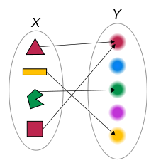
如此當數學家說『函數』 的定義時︰
的定義時︰
假使有兩個集合  和
和  ,將之稱作『定義域』domain 與『對應域』codomain,函數 是
  的子集,並且滿足

,記作  ,『
,『  』是指『恰有一個』,就一點都不奇怪了吧。同樣『二元運算』假使『簡記』成
  ,
, ,是講︰
,是講︰
 ,也是很清晰明白的呀!!


如果仔細考察  ── 比方說
  ──,那麼『函數 』是什麼呢?『變數
  』又是什麼呢?如果從函數定義可以知道『變數』並不是什麼『會變的數』,而是規定在『定義域』或者『對應域』中的『某數』的概念,也就是講在該定義的『集合元素中』談到『每一個』、『有一個』和『恰有一個』…的那樣之『指稱』觀念。這能有什麼困難的嗎?假使設想另一個函數
  ,它的定義域與對應域都和函數 一樣,那麼這兩個函數是一樣還是不一樣的呢?如果說它們是相同的函數,那麼這個所說的『函數』就該是『
 』,其中
』,其中  『變數』只是『命名的』── 函數的輸出之數 ──,而且
  『變數』是『虛名的』── 函數的輸入之數 ──。如果從函數 將『輸入的數』轉換成『輸出的數』的觀點來看,這個『輸入與輸出』本就是 所『固有的』,所以和『輸入與輸出』到底是怎麼『命名』無關的啊!更何況『定義域或對應域』任一也都不必是『數的集合』,這時所講的『函數』或許稱作『函式』比較好,『變數』或該叫做『變元』。其次假使將多個函數『合成』composition,好比『輸出入』的串接,舉例來講,一般數學上表達成
  ,此時假使不補足,
 和
和  ,怕是不能知道這個函數的『結構』是什麼的吧?進一步講『函數』難道不能看成『計算操作子』operator 的概念,定義著什麼是
 、
、 、
、 或
或  的嗎?就像將之這樣定義成︰

,而將函數合成這麼定義為︰

。如此將使『函數』或者『二元運算』的定義域或對應域可以含括『函數』的物項,所以說它是『泛函式』functional 的了。
再者將函式的定義域由一數一物推廣到『有序元組』turple 也是很自然的事,就像講房間裡的『溫度函數』是  一樣,然而這也產生了另一種表達的問題。假想
  、
、  和
和  ,這
,這  兩個函數都是
  函數的『部份』partial 函數,構成了兩個不同的『函數族』。於是在一個運算過程中,這個表達式『
  』究竟是指什麼?是指『』還是指『
 』呢?也許說不定是指『』的呢?難道說『兩平方數之差』本身就沒有意義的嗎??因是之故,邱奇所發展的『λ 記號法』是想要『清晰明白』的『表述』一個『表達式』所說之內容到底是指的什麼。如果使用這個記號法,
 記作︰
記作︰


。那麼之前的  也可以寫成了︰
 。
。
── 說是清晰明白的事理,表達起來卻未必是清楚易懂 ──
─── 摘自《λ 運算︰淵源介紹》


![f\left(\left[ \begin{array}{c} 2 \\ 3 \end{array} \right] \right) = \left[ \begin{array}{c} f(2) \\ f(3) \end{array} \right] = \left[ \begin{array}{c} 4 \\ 9 \end{array} \right], \ \ \ \ (24)](http://www.freesandal.org/wp-content/ql-cache/quicklatex.com-288d1de58c3c6a1e1548bfc0212baf49_l3.png "Rendered by QuickLaTeX.com")


 is just the weighted input to the activation function for neuron
 用大寫字母表示,『向量』
  ,如是
,如是  就是該『矩陣』,第
  就是『行向量』
  個『元素』的了。
 與前一層
與前一層  之『激活』
之『激活』  的關係呢??!!如此可將所謂的『向量函式』
  理解為
理解為  也將順理成章耶!!??
 看成『加』,將
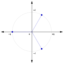
  想為 『乘』。然而『數學』的一般『抽象結構』是由『規則』所『定義』的,很多講的是某個『集合』內之『元素』所具有的『性質』,以及『運算』所滿足的『定律』。這與有沒有人們所『熟悉的』類似結構無關,而且那些『元素』也未必得是個『數』的啊!這或許就是『抽象數學』之所以『困難』的原因。雖然從『純粹』的『邏輯推理』能夠得到『結論』,只不過要是缺乏『經驗性』,人們通常『感覺』不實在、不具體、而且也不安心。就讓我們試著給這個『體』一的比較容易『理解』之結構的『再現』︰設想將
  表現在『複數平面』上,其中
  是『原點』,而
  位在『單位圓』之上,定義如下


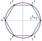
![\because I \bigoplus A \equiv_{rp} \ - \left[ 1 + \left( - \frac{1}{2} + i \frac{\sqrt{3}}{2} \right) \right]](http://www.freesandal.org/wp-content/ql-cache/quicklatex.com-859e9b02e655fe9bdb68a456cf75cb30_l3.png "Rendered by QuickLaTeX.com")


 ,這不就是『
 的『解』
的『解』  的嗎?再徵之以『


 至
至 的冪:
的冪: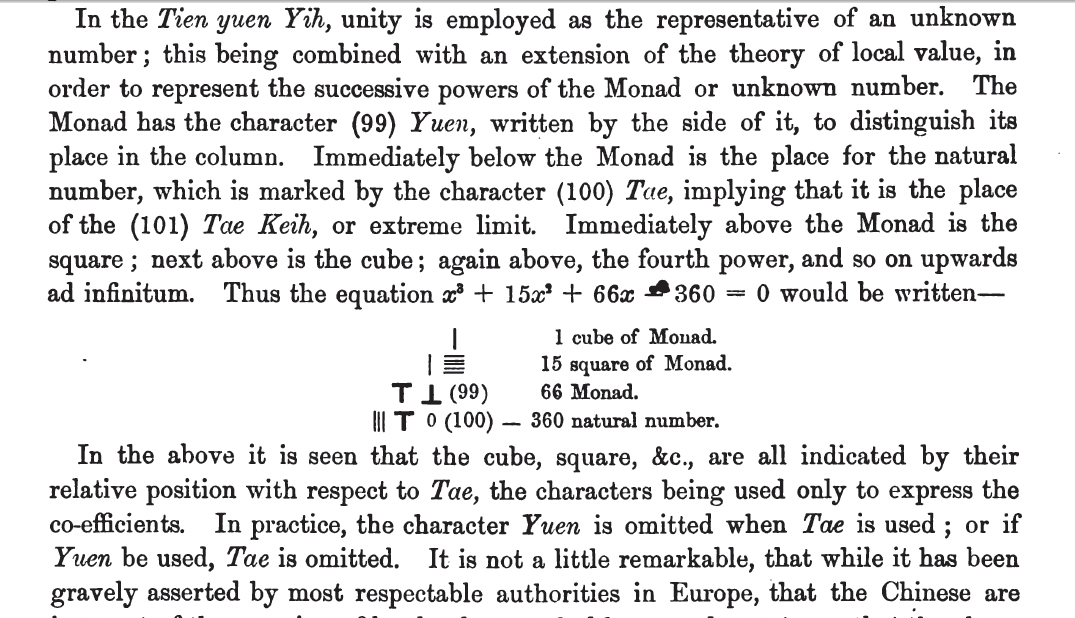

 用天元術表示為:
 項)
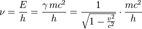
項) 之光量子,攜帶
  的能量 ── 來解釋『


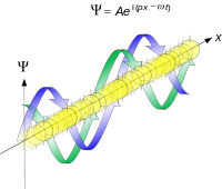
 必須滿足下列條件:
 ,也即
,也即 並單位化
並單位化 ,也即
,也即

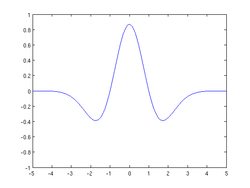
 連續且有一個矩(moment)為0的大整數M,也即對所有整數m<M滿足
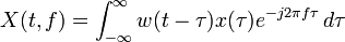
 ,稱作可採納性(admissibility condition),其中
 是
是  的傅立葉轉換。

 的值越大。
的值越大。


 時間,快於
時間,快於 ,其中
,其中 代表數據大小。