在《制器尚象,恆其道。》的文本裡︰
人類如何『創造』呢?在此一篇短文中無法談及全豹,所以串講科學史上幾則逸事略窺一斑。就讓我們從『苯環之夢』談起,
【苯環之夢】
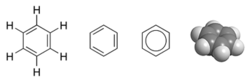
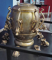
凱庫勒夢到了苯分子是一個環狀結構。
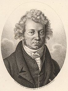
1864年冬,某天德國化學家凱庫勒 Friedrich August Kekulé von Stradonitz 正坐在壁爐前打瞌睡,迷糊中原子們開始飛舞,碳原子串成了鏈,像蛇一般環繞,就像咬著自己的尾巴似的,在他眼前迴旋。 猛然地驚醒後,凱庫勒終於明白了苯分子是一個環狀結構。碳原子們在對稱的六邊形上跳動。
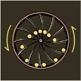
【雜訊放大器】
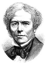
傳聞有一回愛因斯坦突發奇想,想將『雜訊』放大,人們都覺得很奇怪,幹嘛要把『沒用的』雜訊放大?難道愛因斯坦很了解『當其無』嗎︰
『老子道德經 第十一章』
三十輻,共一轂,當其無,有車之用。
埏埴以爲器,當其無,有器之用。
鑿戶牖以爲室,當其無,有室之用。
故有之以爲利,無之以爲用。
或許應該說如果沒有『無所不在』的雜訊,又怎麽能製作『任意頻率』── 放大雜訊,用慮波器選擇所要的頻率 ── 的振盪器呢?恰可比美於所謂的『腦力激盪』之法。
【研究不可能的好處】
達文西之永動機
自古以來,許多人前仆後繼的不斷嘗試想發明『永動機』── 一種能夠 持續運轉工作的機器。今天的熱力學告訴我們這是『不可能』實現的。
既然『不可能』,那『為什麼』要研究呢?首先,熱力學的發展歷史,就是想要證實『永動機』是可能的或是不可能的?其次,過去不可能的,現在還是不可能?牛頓的蘋果如果能量不夠,是飛不出牆,打不到我的;但是量子力學的電子,即使能量依然不夠,卻能穿牆而過── 隧道效應 ──。所以說,不可能未必然是『必然的不可能』。再者,過去也有人曾經說過︰設計高階的電腦語言是『不可能』的,因為人類自己都還『搞不懂』自己怎麽學會語言的,哪又怎能『教得會』電腦呢?答案不言而喻。
專心致志,恆一其道,或許是制器尚象的精粹。比擬︰
『如何制作雷射』
精誠所至 〒 匹配濾波器選擇『所要的』波長的『共振腔』,
金石為開 〒 共振放大後得到 『Laser』。
───
點出了『濾波』概念的重要性。怎麼從錯綜萬象中摘取『所需』?如何自複雜數據裡提煉『所要』??尚難盡『濾波』實務於萬一!略引維基百科若干條例,或可知其理念廣大的乎!!
【布林編程】
Filter (higher-order function)
In functional programming, filter is a higher-order function that processes a data structure (typically a list) in some order to produce a new data structure containing exactly those elements of the original data structure for which a given predicate returns the boolean value true.
【訊號處理】
Filter (signal processing)
In signal processing, a filter is a device or process that removes from a signal some unwanted component or feature. Filtering is a class of signal processing, the defining feature of filters being the complete or partial suppression of some aspect of the signal[clarification needed]. Most often, this means removing some frequencies and not others in order to suppress interfering signals and reduce background noise. However, filters do not exclusively act in the frequency domain; especially in the field of image processing many other targets for filtering exist. Correlations can be removed for certain frequency components and not for others without having to act in the frequency domain.
There are many different bases of classifying filters and these overlap in many different ways; there is no simple hierarchical classification. Filters may be:
- linear or non-linear
- time-invariant or time-variant, also known as shift invariance. If the filter operates in a spatial domain then the characterization is space invariance.
- causal or not-causal: depending if present output depends or not on “future” input; of course, for time related signals processed in real-time all the filters are causal; it is not necessarily so for filters acting on space-related signals or for deferred-time processing of time-related signals.
- analog or digital
- discrete-time (sampled) or continuous-time
- passive or active type of continuous-time filter
- infinite impulse response (IIR) or finite impulse response (FIR) type of discrete-time or digital filter.
【哲學思辨】
Category (Kant)
In Kant‘s philosophy, a category is a pure concept of the understanding. A Kantian category is a characteristic of the appearance of any object in general, before it has been experienced. Kant wrote that “They are concepts of an object in general….”[1] Kant also wrote that, “…pure cоncepts [Categories] of the undеrstanding…apply to objects of intuition in general….”[2] Such a category is not a classificatory division, as the word is commonly used. It is, instead, the condition of the possibility of objects in general,[3] that is, objects as such, any and all objects, not specific objects in particular.
Meaning of “category”
The word comes from the Greek κατηγορία, katēgoria, meaning “that which can be said, predicated, or publicly declared and asserted, about something.” A category is an attribute, property, quality, or characteristic that can be predicated of a thing. “…I remark concerning the categories…that their logical employment consists in their use as predicates of objects.”[4] Kant called them “ontological predicates.”[5]
Aristotle had claimed that the following ten predicates or categories could be asserted of anything in general: substance, quantity, quality, relation, action, affection (passivity), place, time (date), position, and state.
| “ | The Categories, or Predicaments — the former a Greek word, the latter its literal translation in the Latin language — were believed to be an enumeration of all things capable of being named, an enumeration by the summa genera (highest kind), i.e., the most extensive classes into which things could be distributed, which, therefore, were so many highest Predicates, one or other of which was supposed capable of being affirmed with truth of every nameable thing whatsoever. | ” |
These are supposed to be the qualities or attributes that can be affirmed of each and every thing in experience. Any particular object that exists in thought must have been able to have the Categories attributed to it as possible predicates because the Categories are the properties, qualities, or characteristics of any possible object in general. The Categories of Aristotle and Kant are the general properties that belong to all things without expressing the peculiar nature of any particular thing. Kant appreciated Aristotle’s effort, but said that his table was imperfect because ” … as he had no guiding principle, he merely picked them up as they occurred to him…”[7]
The Categories do not provide knowledge of individual, particular objects. Any object, however, must have Categories as its characteristics if it is to be an object of experience. It is presupposed or assumed that anything that is a specific object must possess Categories as its properties because Categories are predicates of an object in general. An object in general does not have all of the Categories as predicates at one time. For example, a general object cannot have the qualitative Categories of reality and negation at the same time. Similarly, an object in general cannot have both unity and plurality as quantitative predicates at once. The Categories of Modality exclude each other. Therefore, a general object cannot simultaneously have the Categories of possibility/impossibility and existence/non–existence as qualities.
Since the Categories are a list of that which can be said of every object, they are related only to human language. In making a verbal statement about an object, a speaker makes a judgment. A general object, that is, every object, has attributes that are contained in Kant’s list of Categories. In a judgment, or verbal statement, the Categories are the predicates that can be asserted of every object and all objects.
───
也許有人會講康德的『範疇說』分明沒提到『濾波』一詞,豈非是胡塞硬套的呢!人的『分別』之心『分類』萬事萬物,『價值』之心『抉擇』想要不要,皆是『心靈濾波器』的耶?若是宇宙一切皆『無差別 』,『範疇』安將能存在的哩??如是當知『濾波』之『結果』正是人所『感知』之『自然』,可一探萬有運作之『心法 』乎!!??
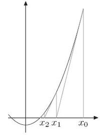
 ,而且如果『初始條件』︰該物位置在原點,速度為零。那麼任意時刻的『速度』是
  ,『位置』為
  。這麼簡易的算術有什麼重要嗎?若是我們可以『追跡物體 』,舉凡相機拍照的防震、手腳運動之練習、肢體平衡復健的監督﹐…… 實有著不勝枚舉之『用途』。然而『微機電』所作的『慣性感測器』 IMU ,一有免不了的『加速度』之『度量誤差』,此誤差在長『時間』的『積累』下將越來『錯誤』越大!再者那個『量測值』只能是『加速度』的『時間序列』
  ,因此
,因此  到
到  時刻間之事也就不得不有『假設』的了!!就像此處問答所說的一樣︰
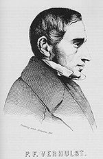


 是某時的人口數,
 是自然成長率,
  是環境承載力。求解後得到
 是初始條件。 Verhulst 將這個函數稱作『logistic function』,於是那個微分方程式也就叫做『 logistic equation』。假使用
  改寫成
改寫成  ,將它『標準化』,取
  與
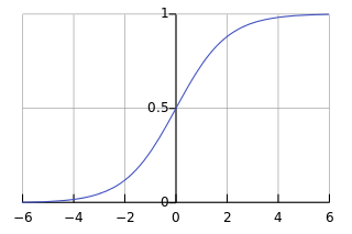
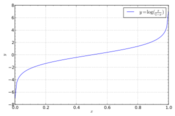
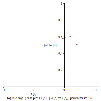
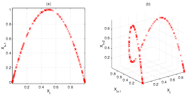
與  ,從左圖的解答來看,
  ,也就是講人口數成長不可能超過環境承載力的啊!
 的反函數,得到
  ,這個反函數被稱之為『Logit』函數,定義為
 和
和  ,或許更能體會『兩極性』的吧!!
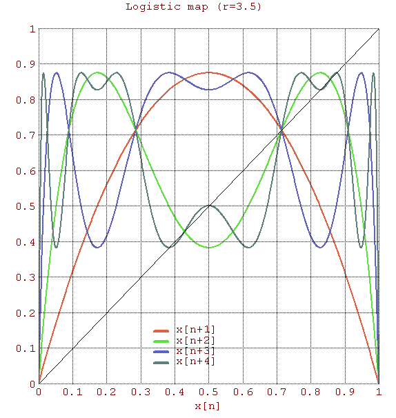
 。這個遞迴關係式很像是『差分版』的『 logistic equation』,竟然是產生『混沌現象』的經典範例。假使說一個『遞迴關係式』有『極限值』
 的話,此時
的話,此時  ,可以得到
,可以得到  ,於是
,於是  或者
或者  。在
。在  之時,『單峰映象』或快或慢的收斂到『零』; 當
  之時,它很快的逼近
  ;於
;於  之時,線性的上下震盪趨近
  也收斂到
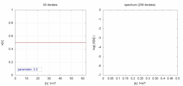
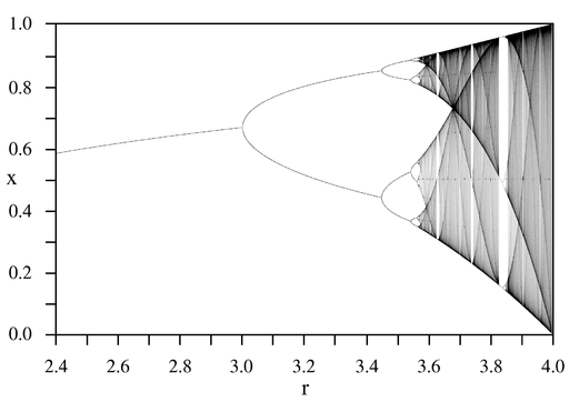
也收斂到  時,對幾乎各個『初始條件』而言,系統開始發生兩值『震盪現象』,而後變成四值、八值、十六值…等等的『持續震盪』;最終於大約
  時,這個震盪現象消失了,系統就步入了所謂的『混沌狀態』的了!!
 的『迭代求值』︰
 。當
。當  ,這個
,這個  就是『定點』,左圖中顯示出不同的
 ![\Delta P(t) = P(t + \Delta t) - P(t) = \left( r P(t) \left[ 1 - P(t) \right] \right) \cdot \Delta t](http://www.freesandal.org/wp-content/ql-cache/quicklatex.com-f862e9b7a6f8941170eb4a06470c1d45_l3.png "Rendered by QuickLaTeX.com") ,假使取
,假使取  ,可以得到
,可以得到 ![P(n + 1) - P(n) = r P(n) \left[ 1 - P(n) \right]](http://www.freesandal.org/wp-content/ql-cache/quicklatex.com-a2bcd9e1f12ec10b81e56b84b4810ef4_l3.png "Rendered by QuickLaTeX.com") ,它的『極限值』
,它的『極限值』  ,根本與
,根本與  看成
看成  ,這樣
,這樣 ![\frac{x[(n+1) \Delta t] - x[n \Delta t]}{\Delta t} = x_{n+1} - x_n](http://www.freesandal.org/wp-content/ql-cache/quicklatex.com-099817979576eb719a1d1161a407d71d_l3.png "Rendered by QuickLaTeX.com") 就說是『速度』的了,於是
就說是『速度』的了,於是  便構成了假想的『
 時,
時, ,因為
,因為  ,所以
,所以  ,於是
,於是  ,因此
,因此  。再者由於『指數項』
  是『偶數』,所以此『符號動力系統』不等速 ──
  來講,它的解是
 是『初始條件』參數,可由
  來決定。假使
  這個『周期函數』,多次『迭代』後就可能產生『極限循環』;要是


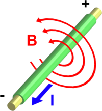
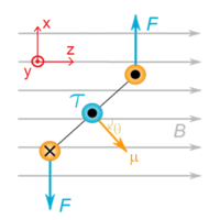

 是『載流導線』
 上的微小『線元素』,
 是那個線元素所載的『電流』量,而
  是『磁常數』。
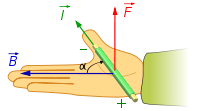
 是圍繞導線的『閉合路徑』,
 是『磁通量感應』強度,
 是此路徑上的微小『線元素』向量,
 是『閉合迴徑』


 and plug in your numbers.

 與『緯度』
與『緯度』  成正比,可以表示為
 的一階導數大於零
  ;但隨著『財富』的增加,『滿足程度』的積累速度卻是不斷下降,正因為『效用函數』之二階導數小於零
  。
。
 ,能產生互斥『結果』
  的『彩票』
的『彩票』  表示成︰
表示成︰ 。
。 ,
, ,或
,或 
 』
』 ,而且
,而且  ,那麼
,那麼  。
。 , 那麼存在一個『機率』
![p\in[0,1]](http://www.freesandal.org/wp-content/ql-cache/quicklatex.com-cd99876237a78fec45ef2ec4cc909f44_l3.png "Rendered by QuickLaTeX.com") ,使得
,使得  。
。 與『機率』
與『機率』 ![p\in(0,1]](http://www.freesandal.org/wp-content/ql-cache/quicklatex.com-2de5bbe9671b75f59e6027e3063c85ec_l3.png "Rendered by QuickLaTeX.com") ,滿足
,滿足  。
。 ,使得
,使得  ,而且對任意兩張『彩票』,如果
  。此處
。此處  代表對
代表對  ,符合
,符合 。
。