自然界中『能量』的『形式』有很多種,不同的『學說‧理論』的歷史的發展,產生了能量的多種『單位』︰
【機械功】︰  是『牛頓‧米』,一『『牛頓‧米』就是一『焦耳』。
【熱能』︰將一公克的水在一大氣壓 ── 101.325 kPa ── 下升高攝氏一度所需要的熱量,叫做一『卡路里』Calorie,簡稱作『卡』,縮寫成 cal。後來的科學家發現水在不同溫度下的比熱容量不同,所以又衍生了許多不同的定義。這就是焦耳所量測的『熱功當量』。一『卡』等於 4.186 『焦耳』。
『電能』︰依據『焦耳定律』  是『安培‧伏特‧秒』,也就是說一『安培‧伏特‧秒』就是一『焦耳』。
所謂的『功率』 power 是指『能量』之『轉換』或者『使用』的『速率』,用單位時間的能量大小來表示。『功率』的『單位』是『瓦特』 W ,假使  是一物理系統在
  時間內所做的功,那麼這段時間內的『平均功率』
  可以由下式給出

。而『瞬時功率』就是當時間  時,『平均功率』的極限值

。也就是講一秒消耗一焦耳的能量就是一『瓦特』,一般所說的『一度電』是指『一千瓦小時』所使用的『電能』多寡,它等於  。
。
從『瞬時功率』 的『定義』,可以推導出
【機械瞬時功率】是  ;
;
【電力瞬時功率】是  。
。
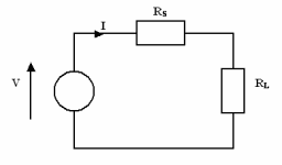

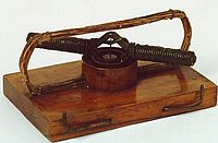
出生於波茨坦的德國物理學家與工程師 Moritz von Jacobi, 一八三五年前往,愛沙尼塔爾圖大學 Tartu Ülikool 任職為教授。自一八三四年起,他就開始研究『磁性馬達』 magnetic motors。據聞一八四零年,於『Die Galvanoplastik』一書中,他提出了『最大功率傳輸理論』Maximum power transfer theorem︰
Maximum power is transferred when the internal resistance of the source equals the resistance of the load, when the external resistance can be varied, and the internal resistance is constant.
。傳聞這個今稱『雅可比定律』早先被『焦耳』誤解為
a system consisting of an electric motor driven by a battery could not be more than 50% efficient since, when the impedances were matched, the power lost as heat in the battery would always be equal to the power delivered to the motor.
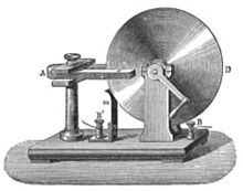
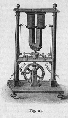
。一八三一年法拉第創造了『Homopolar generator』的『直流發電機』,現今稱之為『Faraday disc』,由於它的『設計構造』,祇能產生很小的『直流電壓』 DC voltage。自此『直流發電機』 dynamo 的『設計改善』就一直持續中。一八三二年,法國的儀器製造商 Hippolyte Pixii 應用『法拉第』的『電磁感應』定律,製造了最早的『交流發電機』alternating current electrical generator。是一種『有電』與『沒電』交替的『電流脈沖』發電機,因此輸出的『平均功率』也很小。一八六六年,適合於工業用的『現代發電機』,最早由英國工程師『瓦利』 C. F. Varley 於十二月二十四日,註冊了『專利』。隔年有兩位『獨立發展者』同時於一月十七日發表了他們的發現。其一是德國『西門子公司』創始人恩斯特‧維爾納‧馮‧西門子 Ernst Werner von Siemens;另一是以『惠斯登電橋』 Wheatstone bridge 稱名於世的英國科學家查爾斯‧惠斯登 Sir Charles Wheatstone。
在有了『發電機』之後,『電功率』有效之『應用』就更顯得重要的了,『最大功率傳輸理論』的『誤解』也將逐漸揭開了『真相』,難道『雅可比』錯了嗎??
一八七八年,就在素有『科學家聖者』scientist-sage 稱號的德國物理學家與醫生赫爾曼‧馮‧亥姆霍茲 Hermann von Helmholtz 推薦下,愛迪生僱用了剛剛取得普林斯頓『碩士學位』的『弗朗西斯‧羅賓‧阿普顿』 Francis Robbins Upton 為助手。由於阿普顿畢業之後曾經跟隨他作過一年的研究,亥姆霍茲深為肯定,又鑑於愛迪生是『自學成家』,所以可能需要有良好『理論技能』的人來協助,因此玉成了這件事情。其後阿普顿成為愛迪生的主要夥伴之一,兩人一起完成了許多發明與創造。其一就是有關『電力工廠』與『配電系統』的研究。一八八零年,愛迪生開始設計『照明系統』,那時的所接受的『智慧』就是使『電樞阻抗』等於『負載電阻』。現今已經不知是愛迪生還是阿普顿覺得這事不對勁。很快的他們了解了『最大功率傳輸』maximum power transfer 和『最大效率』是不同的兩件事,於是便將『發電機』的『電樞阻抗』下降,得到了 90% 的效率。當時美國科技出版業的『專家』嘲諷的說︰就在他事實上作出來的時候,我卻根本作不了。之後大家都知道了這真的是一個『事實』,終究愛迪生或阿普顿幾乎從未因此得到過任何的讚譽。
『雅可比定律』是說當『電壓源』  的『內阻』
的『內阻』  固定的時候,對於『可變動』的『負載電阻』
  來講,假使
來講,假使  這時的『功率傳輸』是『最大值』。
這可以推導如下,依據歐姆定律

,因此

,所以當  就是『功率傳輸』之『最大值』的條件,可以得到
  ,再由二階導數
  的『正、負』號,來判斷『極小、大值』,就可歸結出了 ,這時
  。
。
『焦耳』的『誤解』在於『錯讀』了『 是常數』的『假設』!為什麼呢?假使我們換一個說法,如果 是『固定的』,那麼哪樣的 可以產生『功率傳輸』之『最大值』的呢?此時它的條件變成  ,然而這個條件得到
  而且此時
而且此時  ,所以它並不是合理的『最大值』。進一步的分析,當
  時,
時, ,於是當
,於是當  是合理範圍內的『功率傳輸』之『最大值』,此時
  。這就是當年愛迪生和阿普顿在說的事情啊!!
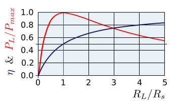
 定義成『負載功率與電源輸出功率的比值』。可以表示成

當  時,『效率』
當  或
或  時,『效率』
當  時,『效率』
─── 精讀與略讀都是重要的閱讀方法,
那何時該略讀的呢?何時又該精讀的呢?
大哉問?? ───
─── 《【SONIC Π】電路學之補充《二》》
固然『學而不思則罔,思而不學則殆。』。
絕非『雜亂無章』之學,『顛三倒四』之思。
如何有系統的學與思?
莫過於上課讀書也!
Circuits and Electronics

A mixed-signal printed circuit board containing both analog and digital components. The board is one component of a 1000-node acoustic beamformer being developed at MIT’s Computer Science and Artificial Intelligence Laboratory. The board contains a pair of microphones, several resistors, capacitors, and digital integrated circuit chips.(Image courtesy of Ken Steele and Anant Agarwal.)
This free electrical engineering textbook provides a series of volumes covering electricity and electronics. The information provided is great for students, makers, and professionals who are looking to refresh or expand their knowledge in this field. These textbooks were written by Tony R. Kuphaldt and released under the Design Science License.
若實有心且又能善用工具︰
/lcapy
Lcapy is a Python package for linear circuit analysis. It uses SymPy
for symbolic mathematics.
Lcapy can analyse circuits described with netlists or by
series/parallel combinations of components.
From version 0.25.0, Lcapy performs more comprehensive circuit
analysis using combinations of DC, AC, and Laplace analysis. This
added functionality has resulted in a slight change of syntax.
cct.R1.V no longer prints the s-domain expression but the
decomposition of a signal into each of the transform domains.
Version 0.25.1 adds time-domain analysis for circuits without reactive
components.
Version 0.26.0 adds noise analysis.
More comprehensive documentation can be found at http://lcapy.elec.canterbury.ac.nz
Circuit analysis
—————-
The circuit is described using netlists, similar to SPICE, with
arbitrary node names (except for the ground node which is labelled 0).
The netlists can be loaded from a file or created at run-time. For
example:
pi@raspberrypi:~ $ python3
Python 3.5.3 (default, Jan 19 2017, 14:11:04)
[GCC 6.3.0 20170124] on linux
Type "help", "copyright", "credits" or "license" for more information.
>>> from lcapy import Circuit
>>> cct = Circuit()
>>> cct.add('Vs 2 0 {5 * u(t)}')
>>> cct.add('Ra 2 1')
>>> cct.add('Rb 1 0')
>>>
>>> cct[1].v
5⋅R_b⋅Heaviside(t)
──────────────────
     Rₐ + R_b
>>> cct[2].v
5⋅Heaviside(t)
>>> cct.Ra.i
5⋅Heaviside(t)
──────────────
   Rₐ + R_b
>>> cct.Ra.v
  5⋅R_b⋅Heaviside(t)
- ────────────────── + 5⋅Heaviside(t)
       Rₐ + R_b
>>>
豈怕天下有難事乎☺