歐式幾何裡並無『座標系』之概念,而是以『全等』關係︰
In geometry, two figures or objects are congruent if they have the same shape and size, or if one has the same shape and size as the mirror image of the other.[1]
More formally, two sets of points are called congruent if, and only if, one can be transformed into the other by an isometry, i.e., a combination of rigid motions, namely a translation, a rotation, and a reflection. This means that either object can be repositioned and reflected (but not resized) so as to coincide precisely with the other object. So two distinct plane figures on a piece of paper are congruent if we can cut them out and then match them up completely. Turning the paper over is permitted.
In elementary geometry the word congruent is often used as follows.[2] The word equal is often used in place of congruent for these objects.
- Two line segments are congruent if they have the same length.
- Two angles are congruent if they have the same measure.
- Two circles are congruent if they have the same diameter.
In this sense, two plane figures are congruent implies that their corresponding characteristics are “congruent” or “equal” including not just their corresponding sides and angles, but also their corresponding diagonals, perimeters and areas.
The related concept of similarity applies if the objects differ in size but not in shape.

An example of congruence. The two triangles on the left are congruent, while the third is similar to them. The last triangle is neither similar nor congruent to any of the others. Note that congruence permits alteration of some properties, such as location and orientation, but leaves others unchanged, like distance and angles. The unchanged properties are called invariants.
研究各類圖形具有種種性質之『不變性』。
參照之前文本所說︰
……
從物理上講,那個三角形就是『剛體』 rigid body ,它在『運動』中保持『形狀』的『不變性』。而且不同觀察者間的『座標變換』可以用
Rigid transformation
In mathematics, a rigid transformation (isometry) of a vector space preserves distances between every pair of points.[1][2] Rigid transformations of the plane R2, space R3, or real n-dimensional space Rn are termed a Euclidean transformation because they form the basis of Euclidean geometry.[3]
The rigid transformations include rotations, translations, reflections, or their combination. Sometimes reflections are excluded from the definition of a rigid transformation by imposing that the transformation also preserve the handedness of figures in the Euclidean space (a reflection would not preserve handedness; for instance, it would transform a left hand into a right hand). To avoid ambiguity, this smaller class of transformations is known as proper rigid transformations (informally, also known as roto-translations). In general, any proper rigid transformation can be decomposed as a rotation followed by a translation, while any rigid transformation can be decomposed as an improper rotation followed by a translation (or as a sequence of reflections).
Any object will keep the same shape and size after a proper rigid transformation.
All rigid transformations are examples of affine transformations. The set of all (proper and improper) rigid transformations is a group called the Euclidean group, denoted E(n) for n-dimensional Euclidean spaces. The set of proper rigid transformation is called special Euclidean group, denoted SE(n).
In kinematics, proper rigid transformations in a 3-dimensional Euclidean space, denoted SE(3), are used to represent the linear and angular displacement of rigid bodies. According to Chasles’ theorem, every rigid transformation can be expressed as a screw displacement.
Formal definition
A rigid transformation is formally defined as a transformation that, when acting on any vector v, produces a transformed vector T(v) of the form
- T(v) = R v + t
where RT = R−1 (i.e., R is an orthogonal transformation), and t is a vector giving the translation of the origin.
A proper rigid transformation has, in addition,
- det(R) = 1
which means that R does not produce a reflection, and hence it represents a rotation (an orientation-preserving orthogonal transformation). Indeed, when an orthogonal transformation matrix produces a reflection, its determinant is –1.
Distance formula
A measure of distance between points, or metric, is needed in order to confirm that a transformation is rigid. The Euclidean distance formula for Rn is the generalization of the Pythagorean theorem. The formula gives the distance squared between two points X and Y as the sum of the squares of the distances along the coordinate axes, that is

where X=(X1, X2, …, Xn) and Y=(Y1, Y2, …, Yn), and the dot denotes the scalar product.
Using this distance formula, a rigid transformation g:Rn→Rn has the property,

─── 摘自《勇闖新世界︰ W!o《卡夫卡村》變形祭︰品味科學‧教具教材‧【專題】 PD‧箱子世界‧留白》
如果依據伽利略『相對性』原理之視角,那麼物理性質也不該因為『觀察者』或『座標系』之不同而有所改變??因是古典力學就得符合『伽利略變換』矣!!
In physics, a Galilean transformation is used to transform between the coordinates of two reference frames which differ only by constant relative motion within the constructs of Newtonian physics. These transformations together with spatial rotations and translations in space and time form the inhomogeneous Galilean group (assumed throughout below). Without the translations in space and time the group is the homogeneous Galilean group. The Galilean group is the group of motions of Galilean relativity action on the four dimensions of space and time, forming the Galilean geometry. This is the passive transformation point of view. The equations below, although apparently obvious, are valid only at speeds much less than the speed of light. In special relativity the Galilean transformations are replaced by Poincaré transformations; conversely, the group contraction in the classical limit c → ∞ of Poincaré transformations yields Galilean transformations.
Galileo formulated these concepts in his description of uniform motion.[1] The topic was motivated by his description of the motion of a ball rolling down a ramp, by which he measured the numerical value for the acceleration of gravity near the surface of the Earth.
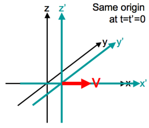
Standard configuration of coordinate systems for Galilean transformations.
只是通常各自有『原點』的『座標系』並不方便以『矩陣』來表達『時空』之『等距同構』
Isometry
In mathematics, an isometry (or congruence, or congruent transformation) is a distance-preserving injective map between metric spaces.[1]
Introduction
Given a metric space (loosely, a set and a scheme for assigning distances between elements of the set), an isometry is a transformation which maps elements to the same or another metric space such that the distance between the image elements in the new metric space is equal to the distance between the elements in the original metric space. In a two-dimensional or three-dimensional Euclidean space, two geometric figures are congruent if they are related by an isometry;[3] the isometry that relates them is either a rigid motion (translation or rotation), or a composition of a rigid motion and a reflection.
Isometries are often used in constructions where one space is embedded in another space. For instance, the completion of a metric space M involves an isometry from M into M’, a quotient set of the space of Cauchy sequences on M. The original space M is thus isometrically isomorphic to a subspace of a complete metric space, and it is usually identified with this subspace. Other embedding constructions show that every metric space is isometrically isomorphic to a closed subset of some normed vector space and that every complete metric space is isometrically isomorphic to a closed subset of some Banach space.
An isometric surjective linear operator on a Hilbert space is called a unitary operator.
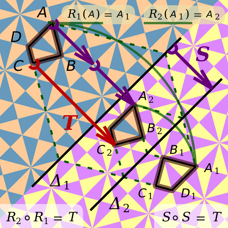
A composition of two opposite isometries is a direct isometry. A reflection in a line is an opposite isometry, like R 1 or R 2 on the image. Translation T is a direct isometry: a rigid motion.[2]
的變換性質,因此借著
在數學裡,齊次坐標(homogeneous coordinates),或投影坐標(projective coordinates)是指一個用於投影幾何裡的坐標系統,如同用於歐氏幾何裡的笛卡兒坐標一般。該詞由奧古斯特·費迪南德·莫比烏斯於1827年在其著作《Der barycentrische Calcul》一書內引入[1][2]。齊次坐標可讓包括無窮遠點的點坐標以有限坐標表示。使用齊次坐標的公式通常會比用笛卡兒坐標表示更為簡單,且更為對稱 。齊次坐標有著廣泛的應用,包括電腦圖形及3D電腦視覺。使用齊次坐標可讓電腦進行仿射變換,並通常,其投影變換能簡單地使用矩陣來表示。
如一個點的齊次坐標乘上一個非零純量,則所得之坐標會表示同一個點。因為齊次坐標也用來表示無窮遠點,為此一擴展而需用來標示坐標之數值比投影空間之維度多一。例如,在齊次坐標裡,需要兩個值來表示在投影線上的一點,需要三個值來表示投影平面上的一點。
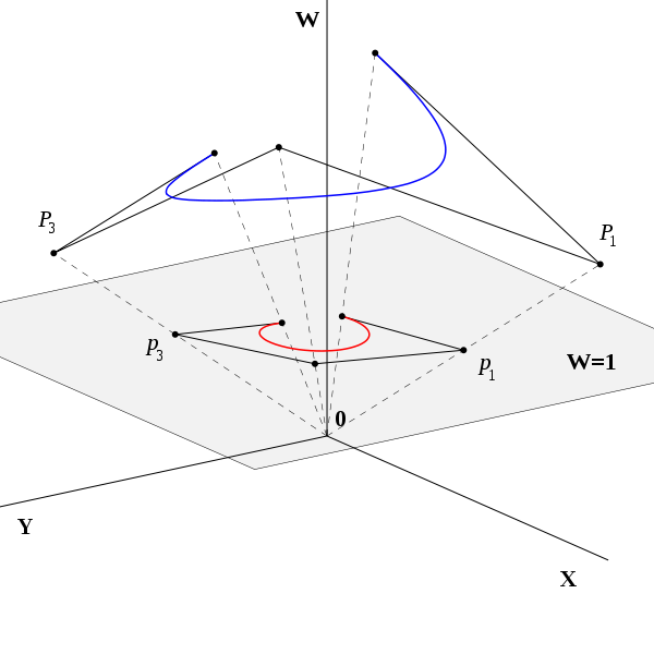
有理貝茲曲線-定義於齊次坐標內的多項式曲線(藍色),以及於平面上的投影-有理曲線(紅色)
來統整論述也就自然而然的了??!!更別說由於雙眼之視覺現象還得走入『仿射變換』的哩!!??
與
的比例同於
及
。


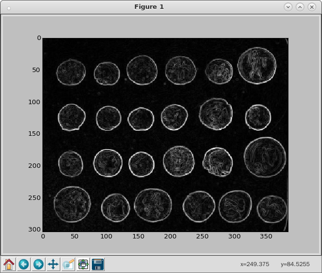
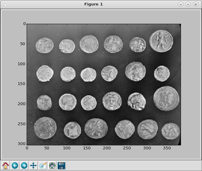
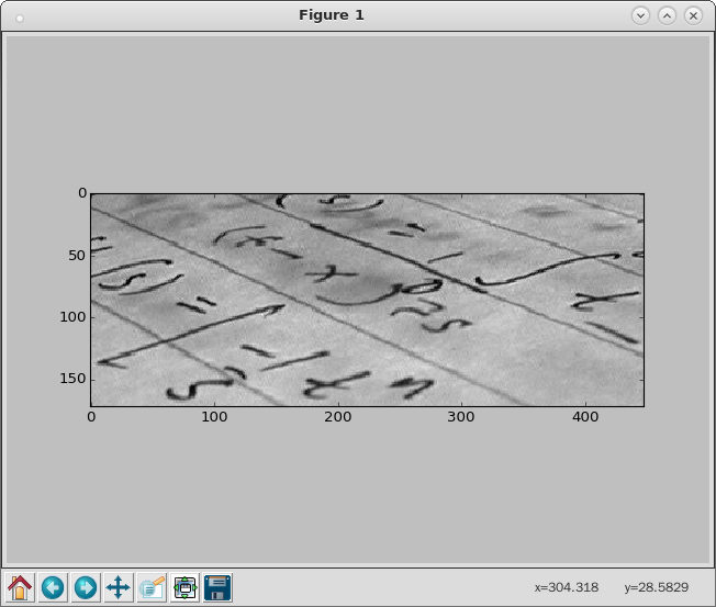
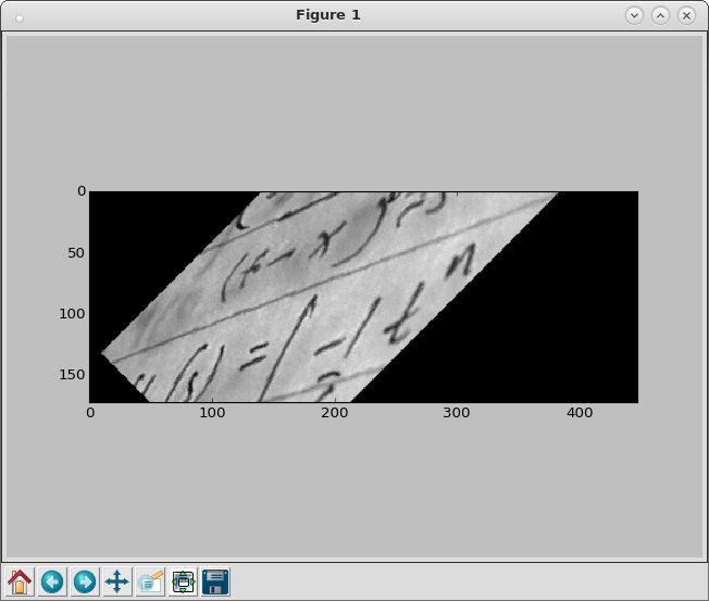
ipython3 Python 3.4.2 (default, Oct 19 2014, 13:31:11) Type "copyright", "credits" or "license" for more information. IPython 2.3.0 -- An enhanced Interactive Python. ? -> Introduction and overview of IPython's features. %quickref -> Quick reference. help -> Python's own help system. object? -> Details about 'object', use 'object??' for extra details. In [1]: from skimage import data, io, filter In [2]: image = data.coins() In [3]: edges = filter.sobel(image) In [4]: io.imshow(edges) In [5]: io.show() In [6]: io.imshow(image) In [7]: io.show() In [8]: 文本 = data.text()
 為『靜止』,『□觀察者』見『○觀察者』
  以『速度』
以『速度』  向右運動,假使他們彼此能『交換資訊』,同意兩者的『原點』相同,那麼他們對『時空現象』或者說『事件』的『位置‧時間』描述滿足
 對『□觀察者』是『靜止』的,然而對『○觀察者』而言,是
  和
和  ,它以『速度』
  與
與  ,對『○觀察者』而言,是
  和
和  也是『同時的』。既然『運動是相對的』,假使我們以『○觀察者』為『靜止』,來作個『伽利略變換』的『物理檢驗』, 那麼
  當是應該的了。也就是說
  ,讀者自己可以『確證』
  它的『正確性』。也可以說『物理之要求』不得不決定了『數學的表達式』的吧!,所謂的『自然律』並不『必須』要『滿足』這種或那種『數學』的耶!!如果說『○觀察者』觀測某一個『星辰』
  用
用  的『速度』向右『直線運動』,那麼這一個『星辰』相對於『□觀察者』的『速度』是什麼的呢?『直覺上』我們認為既然『


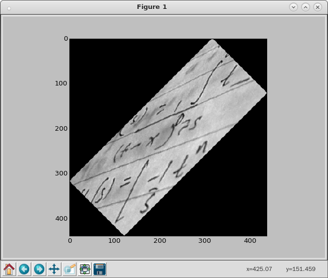
 2 x 2$ 之矩陣豈足以兼顧『平移』和『旋轉』乎 !!??終究還是得進入『
 平移
平移  ,與旋轉放大縮小
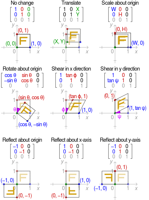
 的仿射映射為

 可被表示為
可被表示為
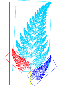
![{\displaystyle {\begin{bmatrix}{\vec {y}}\\1\end{bmatrix}}=\left[{\begin{array}{ccc|c}\,&A&&{\vec {b}}\ \\0&\ldots &0&1\end{array}}\right]{\begin{bmatrix}{\vec {x}}\\1\end{bmatrix}}}](https://wikimedia.org/api/rest_v1/media/math/render/svg/4b3f8dfb50a5d0500891ce899036d73cfd362042)

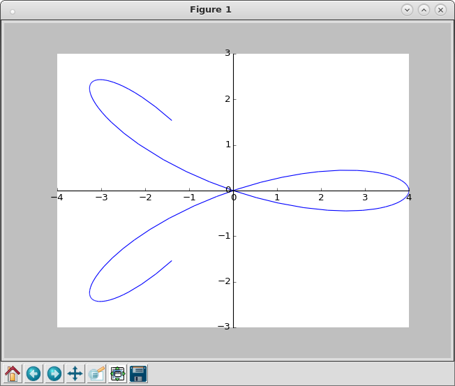
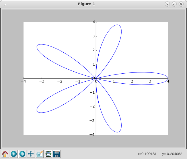
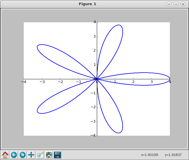
![\begin{array}{rcl} x(t)&=&R\left[(1-k)\cos t+lk\cos \frac{1-k}{k}t\right] ,\\[4pt] y(t)&=&R\left[(1-k)\sin t-lk\sin \frac{1-k}{k}t\right] .\\\end{array}](https://www.freesandal.org/wp-content/ql-cache/quicklatex.com-ea77aa476c55506d41f7e14c0473dc7c_l3.png "Rendered by QuickLaTeX.com")
 是『外大齒輪』的半徑,
 是大小齒輪的『半徑比』
  ,
, 是筆洞所在位置到『內小齒輪』圓心的距離與『內小齒輪』半徑的比值
  。
。

 矩陣之『反矩陣』
 為例,演義這則『伐柯取妻』有趣之事︰

