洋洋灑灑之文,自然成章,根本無可註解。但請跟著 Michael Nielsen 先生來趟發現之旅耶!!
So, what goes wrong when we try to train a deep network?
To answer that question, let’s first revisit the case of a network with just a single hidden layer. As per usual, we’ll use the MNIST digit classification problem as our playground for learning and experimentation*
*I introduced the MNIST problem and data here and here..
If you wish, you can follow along by training networks on your computer. It is also, of course, fine to just read along. If you do wish to follow live, then you’ll need Python 2.7, Numpy, and a copy of the code, which you can get by cloning the relevant repository from the command line:
git clone https://github.com/mnielsen/neural-networks-and-deep-learning.git
If you don’t use git then you can download the data and code here. You’ll need to change into the src subdirectory.
Then, from a Python shell we load the MNIST data:
>>> import mnist_loader
>>> training_data, validation_data, test_data = \
... mnist_loader.load_data_wrapper()
We set up our network:
>>> import network2
>>> net = network2.Network([784, 30, 10])
This network has 784 neurons in the input layer, corresponding to the  pixels in the input image. We use 30 hidden neurons, as well as 10 output neurons, corresponding to the 10 possible classifications for the MNIST digits (‘0’, ‘1’, ‘2’,
  , ‘9’).
Let’s try training our network for 30 complete epochs, using mini-batches of 10 training examples at a time, a learning rate  , and regularization parameter
  . As we train we’ll monitor the classification accuracy on the validation_data*
*Note that the networks is likely to take some minutes to train, depending on the speed of your machine. So if you’re running the code you may wish to continue reading and return later, not wait for the code to finish executing.:
>>> net.SGD(training_data, 30, 10, 0.1, lmbda=5.0,
... evaluation_data=validation_data, monitor_evaluation_accuracy=True)
We get a classification accuracy of 96.48 percent (or thereabouts – it’ll vary a bit from run to run), comparable to our earlier results with a similar configuration.
Now, let’s add another hidden layer, also with 30 neurons in it, and try training with the same hyper-parameters:
>>> net = network2.Network([784, 30, 30, 10])
>>> net.SGD(training_data, 30, 10, 0.1, lmbda=5.0,
... evaluation_data=validation_data, monitor_evaluation_accuracy=True)
This gives an improved classification accuracy, 96.90 percent. That’s encouraging: a little more depth is helping. Let’s add another 30-neuron hidden layer:
>>> net = network2.Network([784, 30, 30, 30, 10])
>>> net.SGD(training_data, 30, 10, 0.1, lmbda=5.0,
... evaluation_data=validation_data, monitor_evaluation_accuracy=True)
That doesn’t help at all. In fact, the result drops back down to 96.57 percent, close to our original shallow network. And suppose we insert one further hidden layer:
>>> net = network2.Network([784, 30, 30, 30, 30, 10])
>>> net.SGD(training_data, 30, 10, 0.1, lmbda=5.0,
... evaluation_data=validation_data, monitor_evaluation_accuracy=True)
The classification accuracy drops again, to 96.53 percent. That’s probably not a statistically significant drop, but it’s not encouraging, either.
This behaviour seems strange. Intuitively, extra hidden layers ought to make the network able to learn more complex classification functions, and thus do a better job classifying. Certainly, things shouldn’t get worse, since the extra layers can, in the worst case, simply do nothing*
*See this later problem to understand how to build a hidden layer that does nothing.
. But that’s not what’s going on.
So what is going on? Let’s assume that the extra hidden layers really could help in principle, and the problem is that our learning algorithm isn’t finding the right weights and biases. We’d like to figure out what’s going wrong in our learning algorithm, and how to do better.
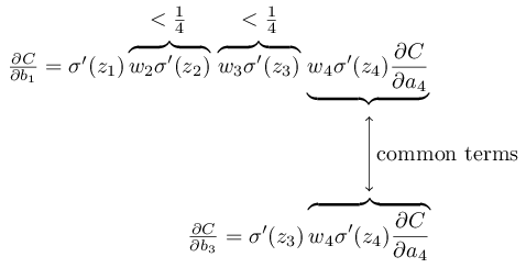
To get some insight into what’s going wrong, let’s visualize how the network learns. Below, I’ve plotted part of a [784,30,30,10] network, i.e., a network with two hidden layers, each containing 30 hidden neurons. Each neuron in the diagram has a little bar on it, representing how quickly that neuron is changing as the network learns. A big bar means the neuron’s weights and bias are changing rapidly, while a small bar means the weights and bias are changing slowly. More precisely, the bars denote the gradient  for each neuron, i.e., the rate of change of the cost with respect to the neuron’s bias. Back in Chapter 2 we saw that this gradient quantity controlled not just how rapidly the bias changes during learning, but also how rapidly the weights input to the neuron change, too. Don’t worry if you don’t recall the details: the thing to keep in mind is simply that these bars show how quickly each neuron’s weights and bias are changing as the network learns.
To keep the diagram simple, I’ve shown just the top six neurons in the two hidden layers. I’ve omitted the input neurons, since they’ve got no weights or biases to learn. I’ve also omitted the output neurons, since we’re doing layer-wise comparisons, and it makes most sense to compare layers with the same number of neurons. The results are plotted at the very beginning of training, i.e., immediately after the network is initialized. Here they are*
*The data plotted is generated using the program generate_gradient.py. The same program is also used to generate the results quoted later in this section.:
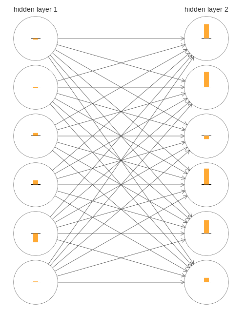
The network was initialized randomly, and so it’s not surprising that there’s a lot of variation in how rapidly the neurons learn. Still, one thing that jumps out is that the bars in the second hidden layer are mostly much larger than the bars in the first hidden layer. As a result, the neurons in the second hidden layer will learn quite a bit faster than the neurons in the first hidden layer. Is this merely a coincidence, or are the neurons in the second hidden layer likely to learn faster than neurons in the first hidden layer in general?
To determine whether this is the case, it helps to have a global way of comparing the speed of learning in the first and second hidden layers. To do this, let’s denote the gradient as  , i.e., the gradient for the
  th neuron in the
  th layer*
*Back in Chapter 2 we referred to this as the error, but here we’ll adopt the informal term “gradient”. I say “informal” because of course this doesn’t explicitly include the partial derivatives of the cost with respect to the weights,  .
.
. We can think of the gradient  as a vector whose entries determine how quickly the first hidden layer learns, and
  as a vector whose entries determine how quickly the second hidden layer learns. We’ll then use the lengths of these vectors as (rough!) global measures of the speed at which the layers are learning. So, for instance, the length
  measures the speed at which the first hidden layer is learning, while the length
  measures the speed at which the second hidden layer is learning.
With these definitions, and in the same configuration as was plotted above, we find  and
and  . So this confirms our earlier suspicion: the neurons in the second hidden layer really are learning much faster than the neurons in the first hidden layer.
What happens if we add more hidden layers? If we have three hidden layers, in a [784,30,30,30,10] network, then the respective speeds of learning turn out to be 0.012, 0.060, and 0.283. Again, earlier hidden layers are learning much slower than later hidden layers. Suppose we add yet another layer with 30 hidden neurons. In that case, the respective speeds of learning are 0.003, 0.017, 0.070, and 0.285. The pattern holds: early layers learn slower than later layers.
We’ve been looking at the speed of learning at the start of training, that is, just after the networks are initialized. How does the speed of learning change as we train our networks? Let’s return to look at the network with just two hidden layers. The speed of learning changes as follows:
 To generate these results, I used batch gradient descent with just 1,000 training images, trained over 500 epochs. This is a bit different than the way we usually train – I’ve used no mini-batches, and just 1,000 training images, rather than the full 50,000 image training set. I’m not trying to do anything sneaky, or pull the wool over your eyes, but it turns out that using mini-batch stochastic gradient descent gives much noisier (albeit very similar, when you average away the noise) results. Using the parameters I’ve chosen is an easy way of smoothing the results out, so we can see what’s going on.
In any case, as you can see the two layers start out learning at very different speeds (as we already know). The speed in both layers then drops very quickly, before rebounding. But through it all, the first hidden layer learns much more slowly than the second hidden layer.
What about more complex networks? Here’s the results of a similar experiment, but this time with three hidden layers (a [784,30,30,30,10] network):
 Again, early hidden layers learn much more slowly than later hidden layers. Finally, let’s add a fourth hidden layer (a [784,30,30,30,30,10] network), and see what happens when we train:
 Again, early hidden layers learn much more slowly than later hidden layers. In this case, the first hidden layer is learning roughly 100 times slower than the final hidden layer. No wonder we were having trouble training these networks earlier!
We have here an important observation: in at least some deep neural networks, the gradient tends to get smaller as we move backward through the hidden layers. This means that neurons in the earlier layers learn much more slowly than neurons in later layers. And while we’ve seen this in just a single network, there are fundamental reasons why this happens in many neural networks. The phenomenon is known as the vanishing gradient problem*
*See Gradient flow in recurrent nets: the difficulty of learning long-term dependencies, by Sepp Hochreiter, Yoshua Bengio, Paolo Frasconi, and Jürgen Schmidhuber (2001). This paper studied recurrent neural nets, but the essential phenomenon is the same as in the feedforward networks we are studying. See also Sepp Hochreiter’s earlier Diploma Thesis, Untersuchungen zu dynamischen neuronalen Netzen (1991, in German)..
Why does the vanishing gradient problem occur? Are there ways we can avoid it? And how should we deal with it in training deep neural networks? In fact, we’ll learn shortly that it’s not inevitable, although the alternative is not very attractive, either: sometimes the gradient gets much larger in earlier layers! This is the exploding gradient problem, and it’s not much better news than the vanishing gradient problem. More generally, it turns out that the gradient in deep neural networks is unstable, tending to either explode or vanish in earlier layers. This instability is a fundamental problem for gradient-based learning in deep neural networks. It’s something we need to understand, and, if possible, take steps to address.
One response to vanishing (or unstable) gradients is to wonder if they’re really such a problem. Momentarily stepping away from neural nets, imagine we were trying to numerically minimize a function  of a single variable. Wouldn’t it be good news if the derivative
  was small? Wouldn’t that mean we were already near an extremum? In a similar way, might the small gradient in early layers of a deep network mean that we don’t need to do much adjustment of the weights and biases?
Of course, this isn’t the case. Recall that we randomly initialized the weight and biases in the network. It is extremely unlikely our initial weights and biases will do a good job at whatever it is we want our network to do. To be concrete, consider the first layer of weights in a [784,30,30,30,10] network for the MNIST problem. The random initialization means the first layer throws away most information about the input image. Even if later layers have been extensively trained, they will still find it extremely difficult to identify the input image, simply because they don’t have enough information. And so it can’t possibly be the case that not much learning needs to be done in the first layer. If we’re going to train deep networks, we need to figure out how to address the vanishing gradient problem.
───
此一『梯度消失問題』之提出
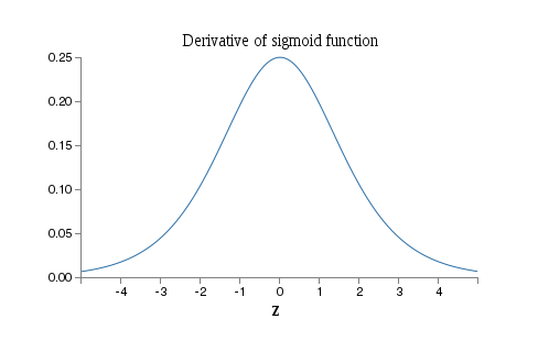
In machine learning, the vanishing gradient problem is a difficulty found in training artificial neural networks with gradient-based learning methods and backpropagation. In such methods, each of the neural network’s weights receives an update proportional to the gradient of the error function with respect to the current weight in each iteration of training. Traditional activation functions such as the hyperbolic tangent function have gradients in the range (−1, 1) or [0, 1), and backpropagation computes gradients by the chain rule. This has the effect of multiplying n of these small numbers to compute gradients of the “front” layers in an n-layer network, meaning that the gradient (error signal) decreases exponentially with n and the front layers train very slowly.
With the advent of the back-propagation algorithm in the 1970s, many researchers tried to train supervised deep artificial neural networks from scratch, initially with little success. Sepp Hochreiter‘s diploma thesis of 1991[1][2] formally identified the reason for this failure in the “vanishing gradient problem”, which not only affects many-layered feedforward networks, but also recurrent neural networks. The latter are trained by unfolding them into very deep feedforward networks, where a new layer is created for each time step of an input sequence processed by the network.
When activation functions are used whose derivatives can take on larger values, one risks encountering the related exploding gradient problem.
───
石破天驚,其人或將永垂神經網絡史乎??

此一『扣鐘之問』,當真是大扣大鳴也!!??
有時候『問』一個『好問題』,勝過『讀』萬卷『答案書』。就讓我們從了解什麼是『好問題』開始吧︰
已故的英國哲學家菲利帕‧福特 Philippa Foot,她於一九六七年發表了一篇名為《堕胎問题和教條雙重影響》論文,當中提出了『電車問題』,用來『批判』時下倫理哲學中之主流思想,尤其是功利主義的觀點︰
大部分之道德判斷都是依據『為最多的人謀取最大之利益』的『原则』而決定的。
她的原文引用如下︰
Suppose that a judge or magistrate is faced with rioters demanding that a culprit be found guilty for a certain crime and threatening otherwise to take their own bloody revenge on a particular section of the community. The real culprit being unknown, the judge sees himself as able to prevent the bloodshed only by framing some innocent person and having him executed.
Beside this example is placed another in which a pilot whose aeroplane is about to crash is deciding whether to steer from a more to a less inhabited area.
To make the parallel as close as possible it may rather be supposed that he is the driver of a runaway tram which he can only steer from one narrow track on to another; five men are working on one track and one man on the other; anyone on the track he enters is bound to be killed. In the case of the riots the mob have five hostages, so that in both examples the exchange is supposed to be one man’s life for the lives of five.
設想一個法官或推事正面對著暴徒的要求,有個罪犯必須為某犯行認罪服法,否則他們將自行報復血洗這個社區的特定區域 。然而真正的犯行者未明,法官觀察到自己似能阻止這場血洗,只要將無辜者框陷處決就好。
除了這個例子之外,另一就是︰一位即將墬機的飛行員要如何決定導向哪個較多還是較少人居住的地方呢。
為了盡可能平行立論,就這樣假想吧︰某人駕駛一輛即將出軌的火車,他僅能從這一窄軌導向另一窄軌;一邊有五人正在軌上工作,另一軌上有一人;不論他進入何軌,那軌道上的人全都必死無疑。好比暴動中一暴民挾持五位人質一樣,當下的兩個例子中都是如此假設一命與五命之兌換。
這個倫理學之『難題』現今有許多不同的類似之『版本』,也許是因為它是這個領域中最為知名的『思想實驗』之一的罷!!
美籍匈牙利的大數學家 George Pólya 寫過一本《怎樣解題》的書,書中強調解題的『第一步』是『了解問題』是什麼?問題的『限制條件』又是什麼?『 概念定義』有沒有『歧義』? 能不能『改寫重述』這個問題的呢?如果『解題者』能這樣作,那就是『思過半已』。
─── 摘自《勇闖新世界︰ 《 pyDatalog 》 導引《十》豆鵝狐人之問題篇》
 來計算
來計算  ,將等於
,將等於 ![\frac{1 - x^m}{1 - x^n} = (1 - x^m) \left[1 + (x^n) + { (x^n) }^2 + { (x^n) } ^3 + \cdots \right]](https://www.freesandal.org/wp-content/ql-cache/quicklatex.com-267693e0c63cf366454627fa281b8762_l3.png "Rendered by QuickLaTeX.com")
 ,那麼
,那麼  難道不應該『等於』
  的嗎?一七四三年時,『伯努利』正因此而反對『歐拉』所講的『可加性』說法,『同』一個級數怎麼可能有『不同』的『和』的呢??作者不知如果在太空裡,乘坐著『加速度』是
  的太空船,在上面用著『樹莓派』控制的『奈米手』來擲『骰子』,是否一定能得到『相同點數』呢?難道說『牛頓力學』不是只要『初始態』是『相同』的話,那個『骰子』的『軌跡』必然就是『一樣』的嗎??據聞,法國籍義大利裔大數學家『約瑟夫 ‧拉格朗日』伯爵 Joseph Lagrange 倒是有個『說法』︰事實上,對於『不同』的
  來講, 從『幂級數』來看,那個
  ,這就與
,這就與  ,擺放到『複數平面』之『單位圓』上來『研究』,輔之以『歐拉公式』
  ,或許可以略探『可加性』理論的『意指』。當
  時,
時, ,雖然
,雖然  ,我們假設那個『幾何級數』 會收斂,於是得到
 ,所以
,所以  以及
以及  。如果我們用
  來『代換』, 此時
  ,可以得到【一】
  和【二】
和【二】  。要是在【一】式中將
  設為『零』的話,我們依然會有
  ;要是驗之以【二】式,當
  時,原式可以寫成
  。如此看來
。如此看來  的『形式運算』,可能是有更深層的『關聯性』的吧!!
 ,此時令
,此時令  ,就得到
,就得到  。如果把【一】式改寫成
  然後對
然後對  ,並將變數
,並將變數  改回
改回  ;再做一次 作『逐項積分』
  ,於是當
,於是當  時,
時, 。然而
。然而 ![1 + \frac{1}{3^2} + \frac{1}{5^2} + \cdots = [1 + \frac{1}{2^2} + \frac{1}{3^2} + \frac{1}{4^2} + \frac{1}{5^2} + \cdots] - [\frac{1}{2^2} + \frac{1}{4^2} + \frac{1}{6^2} + \cdots]](https://www.freesandal.org/wp-content/ql-cache/quicklatex.com-35ef82d73824b7f5cf73ce7044db5497_l3.png "Rendered by QuickLaTeX.com")
![=[1 - \frac{1}{4}][1 + \frac{1}{2^2} + \frac{1}{3^2} + \frac{1}{4^2} + \frac{1}{5^2} + \cdots]](https://www.freesandal.org/wp-content/ql-cache/quicklatex.com-f4f905e0741cad75df0ab00e96e99b94_l3.png "Rendered by QuickLaTeX.com") ,如此我們就能得到了『巴塞爾問題』的答案
,如此我們就能得到了『巴塞爾問題』的答案  。那麼
。那麼 減
減 等於
等於 ,所以
,所以  。
。 之『極限』
之『極限』  存在,
存在,  能不滿足
能不滿足  的嗎?或者可以是
  的呢?即使又已知
  ,還是說可能會發生
  的哩!若是說那些都不會發生,所謂的『可加性』的『概念』應當就可以看成『擴大』且包含『舊有』的『級數的極限』 的『觀點』的吧!也許我們應當使用別種『記號法』來『表達』它,以免像直接寫作
  般的容易引起『誤解 』,畢竟是也存在著多種『可加法』的啊!至於說那些『可加法』的『意義詮釋』,就看『使用者』的吧!!
 除了
除了  是『不連續』外,而『幾何級數』
  『都收斂』,因是
  。也就是說『連續性』、『泰勒展開式』與『級數求和』等等之間有極深的『聯繫 』,事實上它也與『定點理論』
  之『關係』微妙的很啊!!
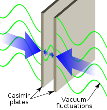

 的『問題』,這也就是說『平均』有『多少』各種能量的『光子?』所參與
  的『問題』?據知『卡西米爾』用『歐拉』等之『可加法』,得到了
  。
。 代表『吸引力』,而今早也已經『證實』的了,真不知『宇宙』是果真先就有『計畫』的嗎?還是說『人們』自己還在『幻想』的呢??
 early in training, substantially slowing down learning. They suggested some alternative activation functions, which appear not to suffer as much from this saturation problem.
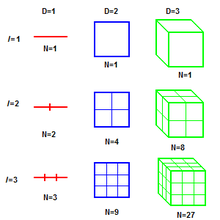

 尺,量一條線段,得到
  ── 單位刻度 ──,如果有另一根
  的尺,它的單位刻度
  是
是 倍,也就是說
  ,那用這
,那用這 。同樣的如果
  ,那用
,那用 ,這樣那
,這樣那 兩尺的度量之數值比
  。
。 的︰
的︰
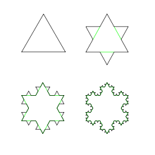
 的 △,到第
  步時︰
步時︰


 ,那時的總周長
  。
。


 . So, for instance, we want


 、
、 、
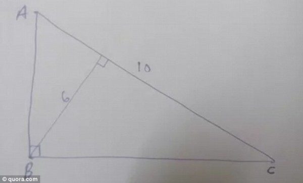
、 ,這個『底之高』
  與『底』相交於
  和
和  兩部份。則有


 、
、 構成『二次方程式』

 。故知此『題意』之直角三角形『不存在』。