從『聯立方程式』 Simultaneous equations 、『線性方程組』 System of linear equations 、『矩陣』 Matrix 、『行列式』 Determinant …… 觀之,『高斯消去法』 Gaussian Elimination 歷史
History
The method of Gaussian elimination appears in the Chinese mathematical text Chapter Eight Rectangular Arrays of The Nine Chapters on the Mathematical Art. Its use is illustrated in eighteen problems, with two to five equations. The first reference to the book by this title is dated to 179 CE, but parts of it were written as early as approximately 150 BCE.[1][2] It was commented on by Liu Hui in the 3rd century.
The method in Europe stems from the notes of Isaac Newton.[3][4] In 1670, he wrote that all the algebra books known to him lacked a lesson for solving simultaneous equations, which Newton then supplied. Cambridge University eventually published the notes as Arithmetica Universalis in 1707 long after Newton left academic life. The notes were widely imitated, which made (what is now called) Gaussian elimination a standard lesson in algebra textbooks by the end of the 18th century. Carl Friedrich Gauss in 1810 devised a notation for symmetric elimination that was adopted in the 19th century by professional hand computers to solve the normal equations of least-squares problems.[5] The algorithm that is taught in high school was named for Gauss only in the 1950s as a result of confusion over the history of the subject.[6]
Some authors use the term Gaussian elimination to refer only to the procedure until the matrix is in echelon form, and use the term Gauss-Jordan elimination to refer to the procedure which ends in reduced echelon form. The name is used because it is a variation of Gaussian elimination as described by Wilhelm Jordan in 1888. However, the method also appears in an article by Clasen published in the same year. Jordan and Clasen probably discovered Gauss–Jordan elimination independently.[7]
久遠矣。或許很多人不曉此法漢代《九章算術》中已有,甚或不知作注的『Liu Hui』劉徽是何許人也!!而後歷經數百代凝鑄成
線性代數
線性代數是關於向量空間和線性映射的一個數學分支。它包括對線、面和子空間的研究,同時也涉及到所有的向量空間的一般性質。
坐標滿足滿足線性方程的點集形成 n 維空間中的一個超平面。n 個超平面相交於一點的條件是線性代數研究的一個重要焦點。此項研究源於包含多個未知數的線性方程組。這樣的方程組可以很自然地表示為矩陣和向量的形式。[1][2]
線性代數既是純數學也是應用數學的核心。例如,放寬向量空間的公理就產生了抽象代數,也就出現了若干推廣。泛函分析研究無窮維情形的向量空間理論。線性代數與微積分結合,使得微分方程線性系統的求解更加便利。 線性代數的理論已被泛化為算子理論。
線性代數的方法還用在解析幾何、工程、物理、自然科學、計算機科學、計算機動畫和社會科學(尤其是經濟學)中。由於線性代數是一套完善的理論,非線性數學模型通常可以被近似為線性模型。
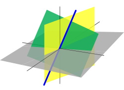
三維歐氏空間R3是一個向量空間,而通過原點的線及平面是R3的向量子空間
歷史
線性代數的研究最初出現於對行列式的研究上。行列式當時被用來求解線性方程組。萊布尼茨在1693年使用了行列式。隨後,加布里爾·克拉默在1750年推導出求解線性方程組的克萊姆法則。然後,高斯利用高斯消元法發展出求解線性系統的理論。這也被列為大地測量學的一項進展。[3][4]
現代線性代數的歷史可以上溯到19世紀中期的英國。1843年,哈密頓發現了四元數。1844年,赫爾曼·格拉斯曼發表了他的著作《線性外代數》(Die lineare Ausdehnungslehre),包括了今日線性代數的一些主題。1848年,詹姆斯·西爾維斯特引入了矩陣(matrix),該詞是「子宮」的拉丁語。阿瑟·凱萊在研究線性變換時引入了矩陣乘法和轉置的概念。很重要的是,凱萊使用了一個字母來代表一個矩陣,因此將矩陣當做了聚合對象。他也意識到矩陣和行列式之間的聯繫。[3]
不過除了這些早期的文獻以外.線性代數主要是在二十世紀發展的。在抽象代數的環論開發之前,矩陣只有模糊不清的定義。隨著狹義相對論的到來,很多開拓者發現了線性代數的微妙。進一步的,解偏微分方程的克萊姆法則的例行應用導致了大學的標準教育中包括了線性代數。例如,E.T. Copson寫到:
1882年,Hüseyin Tevfik Pasha寫了一本書,名為《線性代數》。[5][6]第一次現代化精確定義向量空間是在1888年,由朱塞佩·皮亞諾提出。在1888年,弗蘭西斯·高爾頓還發起了相關係數的應用。經常有多於一個隨機變量出現並且它們可以互相關。在多變元隨機變量的統計分析中,相關矩陣是自然的工具。所以這種隨機向量的統計研究幫助了矩陣用途的開發。到1900年,一種有限維向量空間的線性變換理論被提出。在20世紀上半葉,許多前幾世紀的想法和方法被總結成抽象代數,線性代數第一次有了它的現代形式。矩陣在量子力學、狹義相對論和統計學上的應用幫助線性代數的主題超越了純數學的範疇。計算機的發展導致更多地研究致力於有關高斯消元法和矩陣分解的有效算法上。線性代數成為了數字模擬和模型的基本工具。[3]
其論述能不厚重乎?其內容能不範圍廣闊耶!系統符號混雜、概念層出不窮、各種分支頻起旁徵博引,豈不目不暇給望洋興嘆呀!!
此處藉著『高斯消去法』例子為範︰
Example of the algorithm
Suppose the goal is to find and describe the set of solutions to the following system of linear equations:

The table below is the row reduction process applied simultaneously to the system of equations, and its associated augmented matrix. In practice, one does not usually deal with the systems in terms of equations but instead makes use of the augmented matrix, which is more suitable for computer manipulations. The row reduction procedure may be summarized as follows: eliminate x from all equations below 

| System of equations | Row operations | Augmented matrix |
|---|---|---|
 |
![\left[{\begin{array}{ccc|c}2&1&-1&8\\-3&-1&2&-11\\-2&1&2&-3\end{array}}\right]](https://wikimedia.org/api/rest_v1/media/math/render/svg/c279270bdbca44706acb79d27400e78e087b08bc) |
|
 |
  |
![\left[{\begin{array}{ccc|c}2&1&-1&8\\0&1/2&1/2&1\\0&2&1&5\end{array}}\right]](https://wikimedia.org/api/rest_v1/media/math/render/svg/5c6b056393df5a20d26cc2a837d080876155353a) |
 |
 |
![\left[{\begin{array}{ccc|c}2&1&-1&8\\0&1/2&1/2&1\\0&0&-1&1\end{array}}\right]](https://wikimedia.org/api/rest_v1/media/math/render/svg/4795004b37edb67b30506b8148fa47a0a7f95106) |
| The matrix is now in echelon form (also called triangular form) | ||
 |
  |
![\left[{\begin{array}{ccc|c}2&1&0&7\\0&1/2&0&3/2\\0&0&-1&1\end{array}}\right]](https://wikimedia.org/api/rest_v1/media/math/render/svg/30d4e61eca6607a30b53dd0302c5f7c7bb1701f5) |
 |
  |
![\left[{\begin{array}{ccc|c}2&1&0&7\\0&1&0&3\\0&0&1&-1\end{array}}\right]](https://wikimedia.org/api/rest_v1/media/math/render/svg/404fbc9e271cb9afc77a915b607efdc350ae7e11) |
 |
  |
![\left[{\begin{array}{ccc|c}1&0&0&2\\0&1&0&3\\0&0&1&-1\end{array}}\right]](https://wikimedia.org/api/rest_v1/media/math/render/svg/d829fa7a9862dd6a11878142ed5715e56316ecb6) |
The second column describes which row operations have just been performed. So for the first step, the x is eliminated from 


Once y is also eliminated from the third row, the result is a system of linear equations in triangular form, and so the first part of the algorithm is complete. From a computational point of view, it is faster to solve the variables in reverse order, a process known as back-substitution. One sees the solution is z = -1, y = 3, and x = 2. So there is a unique solution to the original system of equations.
Instead of stopping once the matrix is in echelon form, one could continue until the matrix is in reduced row echelon form, as it is done in the table. The process of row reducing until the matrix is reduced is sometimes referred to as Gauss-Jordan elimination, to distinguish it from stopping after reaching echelon form.
翻古出新,談談如何用『SymPy』之
‧ Matrices
模組為『工具』,操作
初等矩陣
線性代數中,初等矩陣(又稱為基本矩陣[1])是一個與單位矩陣只有微小區別的矩陣。具體來說,一個n階單位矩陣E經過一次初等行變換或一次初等列變換所得矩陣稱為n階初等矩陣。[2]
操作
初等矩陣分為3種類型,分別對應著3種不同的行/列變換。
- 兩行(列)互換:
-

- 把某行(列)乘以一非零常數:
其中

- 把第i行(列)加上第j行(列)的k倍:

初等矩陣即是將上述3種初等變換應用於一單位矩陣的結果。以下只討論對某行的變換,列變換可以類推。
行互換
這一變換Tij,將一單位矩陣的第i行的所有元素與第j行互換。

性質
 。
。 。與其他相同大小的方陣A亦有一下性質:
 。
。把某行乘以一非零常數
這一變換Ti(m),將第i行的所有元素乘以一非零常數m。

性質
-
- 逆矩陣為
。
- 此矩陣及其逆矩陣均為對角矩陣。
- 其行列式
。故對於一等大方陣A有
。
- 逆矩陣為
把第i行加上第j行的m倍
這一變換Tij(m),將第i行加上第j行的m倍。

性質
-
- 逆矩陣具有性質
。
- 此矩陣及其逆矩陣均為三角矩陣。
。故對於一等大方陣A有:
。
- 逆矩陣具有性質
親自『實證』消去法的精神,體驗用『工具』來『學習』之樂趣吧! !
省思這個『初等』當真可『模擬』紙筆運算嗎??
pi@raspberrypi:~ $ python3
Python 3.4.2 (default, Oct 19 2014, 13:31:11)
[GCC 4.9.1] on linux
Type "help", "copyright", "credits" or "license" for more information.

>>> from sympy import *
>>> init_printing()
>>> a, b, c, d, e, f, g, h, i, m = symbols('a, b, c, d, e, f, g, h, i, m')
>>> M = Matrix([[a, b, c], [d, e, f], [g, h, i]])
>>> M
⎡a  b  c⎤
⎢       ⎥
⎢d  e  f⎥
⎢       ⎥
⎣g  h  i⎦

>>> 二三列交換 = Matrix([[1, 0, 0], [0, 0, 1], [0, 1, 0]])
>>> 二三列交換
⎡1  0  0⎤
⎢       ⎥
⎢0  0  1⎥
⎢       ⎥
⎣0  1  0⎦
>>> 二三列交換 * M
⎡a  b  c⎤
⎢       ⎥
⎢g  h  i⎥
⎢       ⎥
⎣d  e  f⎦

>>> 第二列乘m = Matrix([[1, 0, 0], [0, m, 0], [0, 0, 1]])
>>> 第二列乘m
⎡1  0  0⎤
⎢       ⎥
⎢0  m  0⎥
⎢       ⎥
⎣0  0  1⎦
>>> 第二列乘m * M
⎡ a    b    c ⎤
⎢             ⎥
⎢d⋅m  e⋅m  f⋅m⎥
⎢             ⎥
⎣ g    h    i ⎦

>>> 第三列加第二列乘m = Matrix([[1, 0, 0], [0, 1, 0], [0, m, 1]])
>>> 第三列加第二列乘m
⎡1  0  0⎤
⎢       ⎥
⎢0  1  0⎥
⎢       ⎥
⎣0  m  1⎦
>>> 第三列加第二列乘m * M
⎡   a        b        c   ⎤
⎢                         ⎥
⎢   d        e        f   ⎥
⎢                         ⎥
⎣d⋅m + g  e⋅m + h  f⋅m + i⎦
>>>
或可得『自學』之法哩!!??
>>> AM = Matrix([[2, 1, -1, 8], [-3, -1, 2, -11], [-2, 1, 2, -3]])
>>> AM
⎡2   1   -1   8 ⎤
⎢               ⎥
⎢-3  -1  2   -11⎥
⎢               ⎥
⎣-2  1   2   -3 ⎦

>>> L2加二分之三L1 = Matrix([[1, 0, 0], [3/2, 1, 0], [0, 0, 1]])
>>> L2加二分之三L1
⎡ 1   0  0⎤
⎢         ⎥
⎢1.5  1  0⎥
⎢         ⎥
⎣ 0   0  1⎦

>>> L2加二分之三L1 * AM
⎡2    1   -1    8 ⎤
⎢                 ⎥
⎢0   0.5  0.5  1.0⎥
⎢                 ⎥
⎣-2   1    2   -3 ⎦

>>> L3加上L1 = Matrix([[1, 0, 0], [0, 1, 0], [1, 0, 1]])
>>> L3加上L1
⎡1  0  0⎤
⎢       ⎥
⎢0  1  0⎥
⎢       ⎥
⎣1  0  1⎦

>>> L3加上L1 * AM
⎡2   1   -1   8 ⎤
⎢               ⎥
⎢-3  -1  2   -11⎥
⎢               ⎥
⎣0   2   1    5 ⎦

>>> L3加上L1 * L2加二分之三L1 * AM
⎡2   1   -1    8 ⎤
⎢                ⎥
⎢0  0.5  0.5  1.0⎥
⎢                ⎥
⎣0   2    1    5 ⎦

>>> L2加二分之三L1 * L3加上L1 * AM
⎡2   1   -1    8 ⎤
⎢                ⎥
⎢0  0.5  0.5  1.0⎥
⎢                ⎥
⎣0   2    1    5 ⎦
# ……


 與
與  的線性關係,也知
  ,將
,將 ![python3 Python 3.4.2 (default, Oct 19 2014, 13:31:11) [GCC 4.9.1] on linux Type "help", "copyright", "credits" or "license" for more information. >>> from sympy import * >>> x0, x1, x2, s0, s1, s2, ζ = symbols('x0, x1, x2, s0, s1, s2, ζ') >>> init_printing() >>> R1 = Eq(s0, x0 + x1 + x2) >>> R2 = Eq(s1, x0 + ζ*x1 + ζ**2 * x2) >>> R3 = Eq(s2, x0 + ζ**2 * x1 + ζ*x2) >>> R1 s₀ = x₀ + x₁ + x₂ >>> R2 2 s₁ = x₀ + x₁⋅ζ + x₂⋅ζ >>> R3 2 s₂ = x₀ + x₁⋅ζ + x₂⋅ζ >>> solve([R1,R2,R3],[x0,x1,x2]) ⎧ 2 ⎪ s₀⋅ζ + s₀⋅ζ - s₁ - s₂ -s₀⋅ζ - s₁ + s₂⋅ζ + s₂ -s₀⋅ζ + s₁⋅ζ + s₁ ⎨x₀: ──────────────────────, x₁: ──────────────────────, x₂: ───────────────── ⎪ 2 ⎛ 2 ⎞ ⎛ 2 ⎩ ζ + ζ - 2 ζ⋅⎝ζ + ζ - 2⎠ ζ⋅⎝ζ + ζ - 2 ⎫ - s₂⎪ ─────⎬ ⎞ ⎪ ⎠ ⎭ >>> </pre> <span style="color: #003300;">概念之表達需要練習,由是才易掌握概念的內涵。不同的觀察點,或能設想前人所未想或尚未竟之處。假使嘗試卻為複雜運算所阻,恐是誤解了工具的發明及其使用之目的。因此『SymPy』無法代替你的『思考』也。事實上就算你告知『SymPy』](https://www.freesandal.org/wp-content/ql-cache/quicklatex.com-dce53fbcd6b4e0e808f8d95e86c956c5_l3.png "Rendered by QuickLaTeX.com") {\xi}^2 + \xi +1 =0
{\xi}^2 + \xi +1 =0![有這一關係式,它也不會『自動』幫你化簡成那一表達式矣。要是只想知道答案,幹嘛那麼麻煩耶??!!</span> <pre class="lang:python decode:true">>>> a, b, c, d, x = symbols('a, b, c, d, x') >>> solve(a*x**3 + b*x**2 + c*x + d , x) [-(-3*c/a + b**2/a**2)/(3*(sqrt(-4*(-3*c/a + b**2/a**2)**3 + (27*d/a - 9*b*c/a**2 + 2*b**3/a**3)**2)/2 + 27*d/(2*a) - 9*b*c/(2*a**2) + b**3/a**3)**(1/3)) - (sqrt(-4*(-3*c/a + b**2/a**2)**3 + (27*d/a - 9*b*c/a**2 + 2*b**3/a**3)**2)/2 + 27*d/(2*a) - 9*b*c/(2*a**2) + b**3/a**3)**(1/3)/3 - b/(3*a), -(-3*c/a + b**2/a**2)/(3*(-1/2 - sqrt(3)*I/2)*(sqrt(-4*(-3*c/a + b**2/a**2)**3 + (27*d/a - 9*b*c/a**2 + 2*b**3/a**3)**2)/2 + 27*d/(2*a) - 9*b*c/(2*a**2) + b**3/a**3)**(1/3)) - (-1/2 - sqrt(3)*I/2)*(sqrt(-4*(-3*c/a + b**2/a**2)**3 + (27*d/a - 9*b*c/a**2 + 2*b**3/a**3)**2)/2 + 27*d/(2*a) - 9*b*c/(2*a**2) + b**3/a**3)**(1/3)/3 - b/(3*a), -(-3*c/a + b**2/a**2)/(3*(-1/2 + sqrt(3)*I/2)*(sqrt(-4*(-3*c/a + b**2/a**2)**3 + (27*d/a - 9*b*c/a**2 + 2*b**3/a**3)**2)/2 + 27*d/(2*a) - 9*b*c/(2*a**2) + b**3/a**3)**(1/3)) - (-1/2 + sqrt(3)*I/2)*(sqrt(-4*(-3*c/a + b**2/a**2)**3 + (27*d/a - 9*b*c/a**2 + 2*b**3/a**3)**2)/2 + 27*d/(2*a) - 9*b*c/(2*a**2) + b**3/a**3)**(1/3)/3 - b/(3*a)] </pre> <span style="color: #003300;">所以打算跟隨詞條文本者</span> <span style="color: #808080;">The polynomials <span class="texhtml"><i>s</i><sub>1</sub></span> and <span class="texhtml"><i>s</i><sub>2</sub></span> are not <a style="color: #808080;" title="Symmetric polynomial" href="https://en.wikipedia.org/wiki/Symmetric_polynomial">symmetric functions</a> of the roots: <span class="texhtml"><i>s</i><sub>0</sub></span> is invariant, while the two non-trivial <a style="color: #808080;" title="Cyclic permutation" href="https://en.wikipedia.org/wiki/Cyclic_permutation">cyclic permutations</a> of the roots send <span class="texhtml"><i>s</i><sub>1</sub></span> to <span class="texhtml"><i>ξ</i> <i>s</i><sub>1</sub></span> and <span class="texhtml"><i>s</i><sub>2</sub></span> to <span class="texhtml"><i>ξ</i><sup>2</sup><i>s</i><sub>2</sub></span>, or <span class="texhtml"><i>s</i><sub>1</sub></span> to <span class="texhtml"><i>ξ</i><sup>2</sup><i>s</i><sub>1</sub></span> and <span class="texhtml"><i>s</i><sub>2</sub></span> to <span class="texhtml"><i>ξ</i> <i>s</i><sub>2</sub></span> (depending on which permutation), while transposing <span class="texhtml"><i>x</i><sub>1</sub></span> and <span class="texhtml"><i>x</i><sub>2</sub></span> switches <span class="texhtml"><i>s</i><sub>1</sub></span> and <span class="texhtml"><i>s</i><sub>2</sub></span>; other transpositions switch these roots and multiply them by a power of <span class="texhtml"><i>ξ</i></span>.</span> <span style="color: #808080;">Thus <span class="texhtml"><i>s</i><sub>1</sub><sup>3</sup></span>, <span class="texhtml"><i>s</i><sub>2</sub><sup>3</sup></span> and <span class="texhtml"><i>s</i><sub>1</sub><i>s</i><sub>2</sub></span> are left invariant by the cyclic permutations of the roots, which multiply them by <span class="texhtml"><i>ξ</i><sup>3</sup> = 1</span>. Also <span class="texhtml"><i>s</i><sub>1</sub><i>s</i><sub>2</sub></span> and <span class="texhtml"><i>s</i><sub>1</sub><sup>3</sup> + <i>s</i><sub>2</sub><sup>3</sup></span> are left invariant by the transposition of <span class="texhtml"><i>x</i><sub>1</sub></span> and <span class="texhtml"><i>x</i><sub>2</sub></span> which exchanges <span class="texhtml"><i>s</i><sub>1</sub></span> and <span class="texhtml"><i>s</i><sub>2</sub></span>. As the <a style="color: #808080;" title="Permutation group" href="https://en.wikipedia.org/wiki/Permutation_group">permutation group</a> <span class="texhtml"><i>S</i><sub>3</sub></span> of the roots is generated by these permutations, it follows that <span class="texhtml"><i>s</i><sub>1</sub><sup>3</sup> + <i>s</i><sub>2</sub><sup>3</sup></span> and <span class="texhtml"><i>s</i><sub>1</sub><i>s</i><sub>2</sub></span> are <a style="color: #808080;" title="Symmetric polynomial" href="https://en.wikipedia.org/wiki/Symmetric_polynomial">symmetric functions</a> of the roots and may thus be written as polynomials in the <a style="color: #808080;" title="Elementary symmetric polynomial" href="https://en.wikipedia.org/wiki/Elementary_symmetric_polynomial">elementary symmetric polynomials</a> and thus as <a style="color: #808080;" title="Rational function" href="https://en.wikipedia.org/wiki/Rational_function">rational functions</a> of the coefficients of the equation. Let <span class="texhtml"><i>s</i><sub>1</sub><sup>3</sup> + <i>s</i><sub>2</sub><sup>3</sup> = <i>A</i></span> and <span class="texhtml"><i>s</i><sub>1</sub><i>s</i><sub>2</sub> = <i>B</i></span> in these expressions, which will be explicitly computed below.</span> <span style="color: #808080;">We have that <span class="texhtml"><i>s</i><sub>1</sub><sup>3</sup></span> and <span class="texhtml"><i>s</i><sub>2</sub><sup>3</sup></span> are the two roots of the quadratic equation <span class="texhtml"><i>z</i><sup>2</sup> − <i>Az</i> + <i>B</i><sup>3</sup> = 0</span>. Thus the resolution of the equation may be finished exactly as described for Cardano's method, with <span class="texhtml"><i>s</i><sub>1</sub></span> and <span class="texhtml"><i>s</i><sub>2</sub></span> in place of <span class="texhtml mvar">u</span> and <span class="texhtml mvar">v</span>.</span> <h4><span id="Computation_of_A_and_B" class="mw-headline" style="color: #808080;">Computation of <i>A</i> and <i>B</i></span></h4> <span style="color: #808080;">Setting <span class="texhtml"><i>E</i><sub>1</sub> = <i>x</i><sub>0</sub> + <i>x</i><sub>1</sub> + <i>x</i><sub>2</sub></span>, <span class="texhtml"><i>E</i><sub>2</sub> = <i>x</i><sub>0</sub> <i>x</i><sub>1</sub> + <i>x</i><sub>1</sub> <i>x</i><sub>2</sub> + <i>x</i><sub>2</sub> <i>x</i><sub>0</sub></span> and <span class="texhtml"><i>E</i><sub>3</sub> = <i>x</i><sub>0</sub> <i>x</i><sub>1</sub> <i>x</i><sub>2</sub></span>, the elementary symmetric polynomials, we have, using that <span class="texhtml"><i>ξ</i><sup>3</sup> = 1</span>:</span> <dl><dd><span style="color: #808080;"><img class="mwe-math-fallback-image-inline" src="https://wikimedia.org/api/rest_v1/media/math/render/svg/d73a441c6318997f243434a988e09076a4680dcc" alt="{\displaystyle s_{1}^{3}=x_{0}^{3}+x_{1}^{3}+x_{2}^{3}+3\zeta (x_{0}^{2}x_{1}+x_{1}^{2}x_{2}+x_{2}^{2}x_{0})+3\zeta ^{2}(x_{0}x_{1}^{2}+x_{1}x_{2}^{2}+x_{2}x_{0}^{2})+6x_{0}x_{1}x_{2}\,.}" /></span></dd></dl><span style="color: #808080;">The expression for <span class="texhtml"><i>s</i><sub>2</sub><sup>3</sup></span> is the same with <span class="texhtml"><i>ξ</i></span> and <span class="texhtml"><i>ξ</i><sup>2</sup></span> exchanged. Thus, using <span class="texhtml"><i>ξ</i><sup>2</sup> + <i>ξ</i> = −1</span> we get</span> <dl><dd><span style="color: #808080;"><img class="mwe-math-fallback-image-inline" src="https://wikimedia.org/api/rest_v1/media/math/render/svg/c0080e5f1ab617c00e45ef0f477487e2c2d192c0" alt="A=s_{1}^{3}+s_{2}^{3}=2(x_{0}^{3}+x_{1}^{3}+x_{2}^{3})-3(x_{0}^{2}x_{1}+x_{1}^{2}x_{2}+x_{2}^{2}x_{0}+x_{0}x_{1}^{2}+x_{1}x_{2}^{2}+x_{2}x_{0}^{2})+12x_{0}x_{1}x_{2}\,," /></span></dd></dl><span style="color: #808080;">and a straightforward computation gives</span> <dl><dd><span style="color: #808080;"><img class="mwe-math-fallback-image-inline" src="https://wikimedia.org/api/rest_v1/media/math/render/svg/8c3992a40096a19b340bbb1d25cc640f7da45489" alt="A=s_{1}^{3}+s_{2}^{3}=2E_{1}^{3}-9E_{1}E_{2}+27E_{3}\,." /></span></dd></dl><span style="color: #808080;">Similarly we have</span> <dl><dd><span style="color: #808080;"><img class="mwe-math-fallback-image-inline" src="https://wikimedia.org/api/rest_v1/media/math/render/svg/872816595c1e986b7c91cf46fbb8cad5aea1c540" alt="B=s_{1}s_{2}=x_{0}^{2}+x_{1}^{2}+x_{2}^{2}+(\zeta +\zeta ^{2})(x_{0}x_{1}+x_{1}x_{2}+x_{2}x_{0})=E_{1}^{2}-3E_{2}\,." /></span></dd></dl><span style="color: #808080;">When solving equation <b>(</b><a style="color: #808080;" href="https://en.wikipedia.org/wiki/Cubic_function#math_1">1</a><b>)</b> we have <span class="texhtml"><i>E</i><sub>1</sub> = −<span class="sfrac nowrap"><i>b</i><span class="visualhide">/</span><i>a</i></span></span>, <span class="texhtml"><i>E</i><sub>2</sub> = <span class="sfrac nowrap"><i>c</i><span class="visualhide">/</span><i>a</i></span></span> and <span class="texhtml"><i>E</i><sub>3</sub> = −<span class="sfrac nowrap"><i>d</i><span class="visualhide">/</span><i>a</i></span></span>. With equation <b>(</b><a style="color: #808080;" href="https://en.wikipedia.org/wiki/Cubic_function#math_2">2</a><b>)</b>, we have <span class="texhtml"><i>E</i><sub>1</sub> = 0</span>, <span class="texhtml"><i>E</i><sub>2</sub> = <i>p</i></span> and <span class="texhtml"><i>E</i><sub>3</sub> = −<i>q</i></span> and thus <span class="texhtml"><i>A</i> = −27<i>q</i></span> and <span class="texhtml"><i>B</i> = −3<i>p</i></span>.</span> <span style="color: #808080;">Note that with equation <b>(</b><a style="color: #808080;" href="https://en.wikipedia.org/wiki/Cubic_function#math_2">2</a><b>)</b>, we have <span class="texhtml"><i>x</i><sub>0</sub> = <span class="sfrac nowrap">1<span class="visualhide">/</span>3</span>(<i>s</i><sub>1</sub> + <i>s</i><sub>2</sub>)</span> and <span class="texhtml"><i>s</i><sub>1</sub><i>s</i><sub>2</sub> = −3<i>p</i></span>, while in Cardano's method we have set <span class="texhtml"><i>x</i><sub>0</sub> = <i>u</i> + <i>v</i></span> and <span class="texhtml"><i>uv</i> = −<span class="sfrac nowrap">1<span class="visualhide">/</span>3</span><i>p</i></span>. Thus we have, up to the exchange of <span class="texhtml mvar">u</span> and <span class="texhtml mvar">v</span>, <span class="texhtml"><i>s</i><sub>1</sub> = 3<i>u</i></span> and <span class="texhtml"><i>s</i><sub>2</sub> = 3<i>v</i></span> . In other words, in this case, Cardano's method and Lagrange's method compute exactly the same things, up to a factor of three in the auxiliary variables, the main difference being that Lagrange's method explains why these auxiliary variables appear in the problem.</span> <span style="color: #003300;">還是得自己動動手呢!!??</span> <pre class="lang:python decode:true">pi@raspberrypi:~](https://www.freesandal.org/wp-content/ql-cache/quicklatex.com-ddf5624a99ea817925c2e05bc01976e0_l3.png "Rendered by QuickLaTeX.com") python3
Python 3.4.2 (default, Oct 19 2014, 13:31:11)
[GCC 4.9.1] on linux
Type "help", "copyright", "credits" or "license" for more information.
>>> from sympy import *
>>> x0, x1, x2, ζ = symbols('x0, x1, x2, ζ')
>>> s0 = x0 + x1 + x2
>>> s1 = x0 + ζ*x1 + ζ**2 * x2
>>> s2 = x0 + ζ**2 * x1 + ζ*x2
>>> (s1**2).expand()
x0**2 + 2*x0*x1*ζ + 2*x0*x2*ζ**2 + x1**2*ζ**2 + 2*x1*x2*ζ**3 + x2**2*ζ**4
>>> collect(x0**2 + 2*x0*x1*ζ + 2*x0*x2*ζ**2 + x1**2*ζ**2 + 2*x1*x2 + x2**2*ζ, ζ)
x0**2 + 2*x1*x2 + ζ**2*(2*x0*x2 + x1**2) + ζ*(2*x0*x1 + x2**2)
>>> (s1**3).expand()
x0**3 + 3*x0**2*x1*ζ + 3*x0**2*x2*ζ**2 + 3*x0*x1**2*ζ**2 + 6*x0*x1*x2*ζ**3 + 3*x0*x2**2*ζ**4 + x1**3*ζ**3 + 3*x1**2*x2*ζ**4 + 3*x1*x2**2*ζ**5 + x2**3*ζ**6
>>> collect(x0**3 + 3*x0**2*x1*ζ + 3*x0**2*x2*ζ**2 + 3*x0*x1**2*ζ**2 + 6*x0*x1*x2 + 3*x0*x2**2*ζ + x1**3 + 3*x1**2*x2*ζ + 3*x1*x2**2*ζ**2 + x2**3, ζ)
x0**3 + 6*x0*x1*x2 + x1**3 + x2**3 + ζ**2*(3*x0**2*x2 + 3*x0*x1**2 + 3*x1*x2**2) + ζ*(3*x0**2*x1 + 3*x0*x2**2 + 3*x1**2*x2)
>>> (s1*s2).expand()
x0**2 + x0*x1*ζ**2 + x0*x1*ζ + x0*x2*ζ**2 + x0*x2*ζ + x1**2*ζ**3 + x1*x2*ζ**4 + x1*x2*ζ**2 + x2**2*ζ**3
>>> collect(x0**2 + x0*x1*ζ**2 + x0*x1*ζ + x0*x2*ζ**2 + x0*x2*ζ + x1**2 + x1*x2*ζ + x1*x2*ζ**2 + x2**2, ζ)
x0**2 + x1**2 + x2**2 + ζ**2*(x0*x1 + x0*x2 + x1*x2) + ζ*(x0*x1 + x0*x2 + x1*x2)
>>>
python3
Python 3.4.2 (default, Oct 19 2014, 13:31:11)
[GCC 4.9.1] on linux
Type "help", "copyright", "credits" or "license" for more information.
>>> from sympy import *
>>> x0, x1, x2, ζ = symbols('x0, x1, x2, ζ')
>>> s0 = x0 + x1 + x2
>>> s1 = x0 + ζ*x1 + ζ**2 * x2
>>> s2 = x0 + ζ**2 * x1 + ζ*x2
>>> (s1**2).expand()
x0**2 + 2*x0*x1*ζ + 2*x0*x2*ζ**2 + x1**2*ζ**2 + 2*x1*x2*ζ**3 + x2**2*ζ**4
>>> collect(x0**2 + 2*x0*x1*ζ + 2*x0*x2*ζ**2 + x1**2*ζ**2 + 2*x1*x2 + x2**2*ζ, ζ)
x0**2 + 2*x1*x2 + ζ**2*(2*x0*x2 + x1**2) + ζ*(2*x0*x1 + x2**2)
>>> (s1**3).expand()
x0**3 + 3*x0**2*x1*ζ + 3*x0**2*x2*ζ**2 + 3*x0*x1**2*ζ**2 + 6*x0*x1*x2*ζ**3 + 3*x0*x2**2*ζ**4 + x1**3*ζ**3 + 3*x1**2*x2*ζ**4 + 3*x1*x2**2*ζ**5 + x2**3*ζ**6
>>> collect(x0**3 + 3*x0**2*x1*ζ + 3*x0**2*x2*ζ**2 + 3*x0*x1**2*ζ**2 + 6*x0*x1*x2 + 3*x0*x2**2*ζ + x1**3 + 3*x1**2*x2*ζ + 3*x1*x2**2*ζ**2 + x2**3, ζ)
x0**3 + 6*x0*x1*x2 + x1**3 + x2**3 + ζ**2*(3*x0**2*x2 + 3*x0*x1**2 + 3*x1*x2**2) + ζ*(3*x0**2*x1 + 3*x0*x2**2 + 3*x1**2*x2)
>>> (s1*s2).expand()
x0**2 + x0*x1*ζ**2 + x0*x1*ζ + x0*x2*ζ**2 + x0*x2*ζ + x1**2*ζ**3 + x1*x2*ζ**4 + x1*x2*ζ**2 + x2**2*ζ**3
>>> collect(x0**2 + x0*x1*ζ**2 + x0*x1*ζ + x0*x2*ζ**2 + x0*x2*ζ + x1**2 + x1*x2*ζ + x1*x2*ζ**2 + x2**2, ζ)
x0**2 + x1**2 + x2**2 + ζ**2*(x0*x1 + x0*x2 + x1*x2) + ζ*(x0*x1 + x0*x2 + x1*x2)
>>>


 用『配方法』來求解,應是自然順理成章之事。若從『發現』之『邏輯』來考察這一『思路』莫非源於
  的『形式』之『啟發』耶?如果由二次式函數
  之觀點來看,難到不能平移『座標系』
  ,使之簡化為
  之『形式』乎??一個簡單的例子
  或可說明,如此尋找
  以求簡化方程式的求解,實無攸利也!那個
  矣!!
矣!!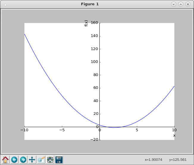

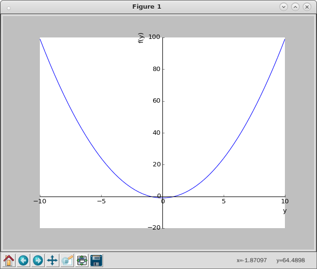

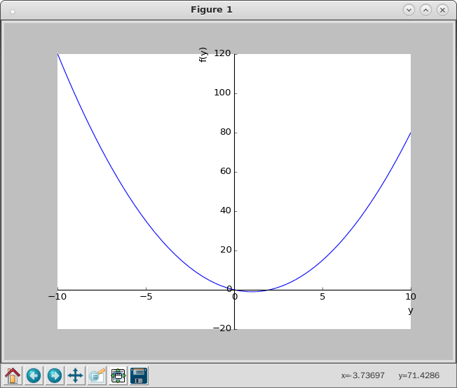

![python3 Python 3.4.2 (default, Oct 19 2014, 13:31:11) [GCC 4.9.1] on linux Type "help", "copyright", "credits" or "license" for more information. >>> from sympy import * >>> x, p, q, α, β, r1, r2 = symbols('x, p, q, α, β, r1, r2') >>> 方程式 = x**2 - 4*x + 3 # Fig 1 >>> plot(方程式) <sympy.plotting.plot.Plot object at 0x75cbba90> >>> y, α = symbols('y, α') >>> 方程式.subs(x, y + α) -4*y - 4*α + (y + α)**2 + 3 >>> init_printing() >>> 方程式.subs(x, y + α) 2 -4⋅y - 4⋅α + (y + α) + 3 >>> 係數式 = collect( (方程式.subs(x, y + α)).expand(), y) >>> 係數式.coeff(y,1) 2⋅α - 4 >>> 係數式.coeff(y,0) 2 α - 4⋅α + 3 >>> factor(方程式.subs(x, y + 2)) (y - 1)⋅(y + 1) >>> factor(方程式.subs(x, y + 1)) y⋅(y - 2) # Fig 2 >>> plot((y - 1)*(y + 1)) Plot object containing: [0]: cartesian line: (y - 1)*(y + 1) for y over (-10.0, 10.0) # Fig 3 >>> plot(y*(y -2)) Plot object containing: [0]: cartesian line: y*(y - 2) for y over (-10.0, 10.0) >>> 二次式 = x**2 + p*x + q >>> 常數項 = collect( (二次式.subs(x, y + α)).expand(), y).coeff(y,0) >>> 常數項 2 p⋅α + q + α >>> </pre> <span style="color: #003300;">此正是拉格朗日能以『單位圓』](https://www.freesandal.org/wp-content/ql-cache/quicklatex.com-7ea59b4a605d1552ad77a1d090f3ed8d_l3.png "Rendered by QuickLaTeX.com") x^2 = 1
x^2 = 1 x = \pm 1
 x^2 + px + q = (x - \alpha)(x -\beta)
 r_1 = \alpha + \betar_2 = \alpha - \beta
 N
N r_2 = \alpha - \beta
 \beta - \alpha
 - r_2
- r_2 \alpha - \beta
 {(\alpha - \beta)}^2 = {(\alpha + \beta)}^2 - 4 \alpha \beta
 r_2
r_2 \alpha = \frac{r_1 + r_2}{2}\beta = \frac{r_1 - r_2}{2}
 \sqrt[4]{-1}
 \sqrt[3]{-1}
 \pm \sqrt{x}
 \sqrt[3]{x}
 \sqrt[n]{x}
 P(x) = \sum \limits_{i=0}^{i=n} c_i \cdot x^i = 0 \ =?= \prod \limits_{k=1}^{k=n} x - x_k
 c_i
c_i x_k
x_k \sqrt{2}
 \sqrt{2}
 \frac{p}{q}
 p
p q
q Q
Q \sqrt{Q}
 \sqrt{Q} = \frac{p}{q}
 p^2 = q^2 \cdot Q
 p, q
p, q p = k \cdot Q
 k, q
k, q q^2 = k^2 \cdot Q
 q = m Q
 p
p q
q Q
Q \sqrt{Q}
 P(x) = x^2 -2 = 0 = (x + \sqrt{2})(x - \sqrt{2})$ 時,這裡所說的『多項式』與『方程式』是一樣的嗎?它們的內在聯繫又是什麼的呢?
 是『多項式』
  的『解』,此處係數
  都是『有理數』。如果我們建構一個『對稱函數』
 應該就是
應該就是  的吧。如果將這些『解』
  ,此處是說上一排的『解』的『位置』用下一排的『解』來『置換』,由於
  函數的特殊『形式』,我們會得到
  。事實上對於任意的『置換』,都會有
  。所以函數
。所以函數  有兩個根
有兩個根  ,
,


 ,和
,和
 與
與  。
。 是方程式的一個根,假設另一個根是
  ,由於
,由於


 。而且
。而且  。也就是說這兩個根是熟悉的
  與
與  。於是一個『對稱函數』
  是
是  的形式﹐那麼必然有另一個根
  是
是  的形式,這就是由於那個『多項式』的係數是『有理數』的原故,它的『二次方根』的解,總是『成對』出現的啊!於是『二次方根』解的個數也必然是『偶數』的了!!
 where
where  is the
  ,其中h和k是
 稱之為
稱之為  的求根公式:
 係數化為1:
 次單位根是
次單位根是
 為
為 。
。 階
階 ,其中
,其中  和
和  。
。 。
。 和
和  ,只有
,只有 
 是
是
 和
和 是本原根。
是本原根。


