當人們閱讀文章時,常常依著原作者的思路,隨其文筆而行。雖覺一路順暢,一旦認真『思考』所讀內容,彷彿無法將那些『字詞』與『概念』連繫起來。比方說,作者讀過 Miller Puckette 先生如下一節講『正弦‧合成』之文本︰
1.5 Synthesizing a sinusoid
In most widely used audio synthesis and processing packages (Csound, Max/MSP, and Pd, for instance), the audio operations are specified as networks of unit generators[Mat69] which pass audio signals among themselves. The user of the software package specifies the network, sometimes called a patch, which essentially corresponds to the synthesis algorithm to be used, and then worries about how to control the various unit generators in time. In this section, we’ll use abstract block diagrams to describe patches, but in the “examples” section (Page 17), we’ll choose a specific implementation environment and show some of the software-dependent details.
To show how to produce a sinusoid with time-varying amplitude we’ll need to introduce two unit generators. First we need a pure sinusoid which is made with an oscillator. Figure 1.5 (part a) shows a pictorial representation of a sinusoidal oscillator as an icon. The input is a frequency (in cycles per second), and the output is a sinusoid of peak amplitude one.
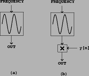 |
Figure 1.5 (part b) shows how to multiply the output of a sinusoidal oscillator by an appropriate scale factor y[n] to control its amplitude. Since the oscillator’s peak amplitude is 1, the peak amplitude of the product is about y[n], assuming y[n] changes slowly enough and doesn’t become negative in value.
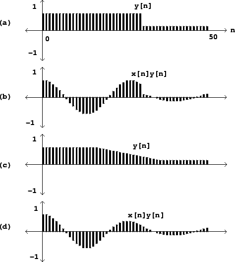 |
Figure 1.6 shows how the sinusoid of Figure 1.1 is affected by amplitude change by two different controlling signals y[n]. The controlling signal shown in part (a) has a discontinuity, and so therefore does the resulting amplitude-controlled sinusoid shown in (b). Parts (c) and (d) show a more gently-varying possibility for y[n] and the result. Intuition suggests that the result shown in (b) won’t sound like an amplitude-varying sinusoid, but instead like a sinusoid interrupted by an audible “pop” after which it continues more quietly. In general, for reasons that can’t be explained in this chapter, amplitude control signals y[n] which ramp smoothly from one value to another are less likely to give rise to parasitic results (such as that “pop”) than are abruptly changing ones.
For now we can state two general rules without justifying them. First, pure sinusoids are the signals most sensitive to the parasitic effects of quick amplitude change. So when you want to test an amplitude transition, if it works for sinusoids it will probably work for other signals as well. Second, depending on the signal whose amplitude you are changing, the amplitude control will need between 0 and 30 milliseconds of “ramp” time—zero for the most forgiving signals (such as white noise), and 30 for the least (such as a sinusoid). All this
also depends in a complicated way on listening levels and the acoustic context.
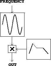
Suitable amplitude control functions y[n] may be made using an envelope generator. Figure 1.7 shows a network in which an envelope generator is used to control the amplitude of an oscillator. Envelope generators vary widely in design, but we will focus on the simplest kind, which generates line segments as shown in Figure 1.6 (part c). If a line segment is specified to ramp between two output values a and b over N samples starting at sample number M , the output is:
The output may have any number of segments such as this, laid end to end, over the entire range of sample numbers n; flat, horizontal segments can be made by setting a = b.
In addition to changing amplitudes of sounds, amplitude control is often used, especially in real-time applications, simply to turn sounds on and off: to turn one off, ramp the amplitude smoothly to zero. Most software synthesis packages also provide ways to actually stop modules from computing samples at all, but here we’ll use amplitude control instead.
The envelope generator dates from the analog era [Str95, p.64] [Cha80, p.90], as does the rest of Figure 1.7; oscillators with controllable frequency were called voltage-controlled oscillators or VCOs, and the multiplication step was done using a voltage-controlled amplifier or VCA [Str95, pp.34-35] [Cha80, pp.84-89].
Envelope generators are described in more detail in Section 4.1.
 |
───
那麼什麼是『振幅控制』呢?又為什麼會有『 pop 』吥吥聲的呢 ??假使以  為『訊號』,用
  表達『振幅控制』,直覺上
  容易理解,因為用它來『控制』當下振幅『大小』 !但是『 gently-varying 』溫和變化意指何事?又將如何解釋下面的兩句話??
First, pure sinusoids are the signals most sensitive to the parasitic effects of quick amplitude change.
……
Second, depending on the signal whose amplitude you are changing, the amplitude control will need between 0 and 30 milliseconds of “ramp” time—zero for the most forgiving signals (such as white noise), and 30 for the least (such as a sinusoid).
───
因此當作者閱讀『原作者』著作時,試圖以下圖的簡單『補丁』
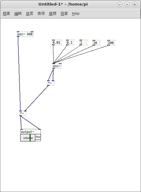
用著原始的『耳朵』來『感覺』文本所說之事。這是因為即使了解了『 line~ 』物件
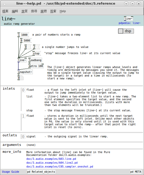
發現用作『聲音開關』不錯,但是在理解『 parasitic effects 』寄生效應上總是不易體會。當時因對 Pd 程式語言認識之不足,所以才會設想那樣奇怪的程式!不過  , 還可以透過頻率
  調節訊號『包絡』 envelope 快慢,感覺十分好玩,或許有益於初學者,故特引以為記!!