假使我們閱讀維基百科詞條對『分貝』 dB 的定義︰
分貝(decibel)是量度兩個相同單位之數量比例的單位,主要用於度量聲音強度,常用dB表示。「分」(deci-)指十分之一,個位是「貝」或「貝爾」(bel,紀念發明家亞歷山大·貝爾),但一般只用分貝。
常用的空氣參考聲壓為 = 20 µPa(微帕斯卡) (rms),它通常被認為是人類的最少聽覺響應值(大約是3米以外飛行的蚊子聲音)。最完善的水平測量,測量1帕斯卡等於94分貝聲壓級。在其他介質 ,如水下,1微帕斯卡更為普遍[1] 。這些標準被ANSIS1.1-1994.所收錄[2]。
計算方法
分貝(dB)是十分之一貝爾(B): 1B = 10dB。1貝爾的兩個功率量的比值是10:1,1貝爾的兩個場量的比值是 [3]。場量(field quantity)是諸如電壓、電流、聲壓、電場強度、速度、電荷密度等量值,其平方值在一個線性系統中與功率成比例。功率量(power quantity)是功率值或者直接與功率值成比例的其它量,如能量密度、音強、發光強度等。
分貝的計算,依賴於是功率量還是場量而不同。
兩個信號具有1分貝的差異,那麼其功率比值是1.25892(即 )而幅值之比是1.12202(即
 )[4]。
)[4]。
功率量
考慮功率或者強度(intensity)時, 其比值可以表示為分貝,這是通過把測量值與參考量值之比計算基於10的對數,再乘以10。因此功率值P1與另一個功率值P0之比用分貝表示為LdB[5] :

兩個功率值的比值基於10的對數,就是貝爾(bel)值。兩個功率值之比的分貝值是貝爾值的10倍(或者說,1個分貝是十分之一貝爾)。P1 與P0必須度量同一個數值類型,具有相同的單位。如果在上式中P1 = P0,那麼LdB = 0。如果P1大於P0,那麼LdB是正的;如果P1小於P0,那麼LdB是負的。
重新安排上式可得到計算P1的公式,依據P0與LdB:
 .
.
因為貝爾是10倍的分貝,對應的使用貝爾(LB)的公式為

 .
.
場量
考慮到場(field)的幅值(amplitude)時,通常使用A1(度量到的幅值)的平方與A0(參考幅值)的平方之比。這是因為對於大多數應用,功率與幅值的平方成比例,並期望對同一應用採取功率計算的分貝與用場的幅值計算的分貝相等。因此使用下述場量的分貝定義:
 與
與 相等,這是由於對數的性質。
上述公式可寫成:
電子電路中,阻抗不變時,耗散功率通常與電壓或電流的平方成正比。以電壓為例,有下述方程:

其中V1是電壓的測量值,V0是指定的參考電壓,GdB是用分貝表示的功率增益。類似的公式對電流也成立。
───
又考察了什麼是『對數尺度』︰
Logarithmic scale
Scientific quantities are often expressed as logarithms of other quantities, using a logarithmic scale. For example, the decibel is a unit of measurement associated with logarithmic-scale quantities. It is based on the common logarithm of ratios—10 times the common logarithm of a power ratio or 20 times the common logarithm of a voltage ratio. It is used to quantify the loss of voltage levels in transmitting electrical signals,[66] to describe power levels of sounds in acoustics,[67] and the absorbance of light in the fields of spectrometry and optics. The signal-to-noise ratio describing the amount of unwanted noise in relation to a (meaningful) signal is also measured in decibels.[68] In a similar vein, the peak signal-to-noise ratio is commonly used to assess the quality of sound and image compression methods using the logarithm.[69]
The strength of an earthquake is measured by taking the common logarithm of the energy emitted at the quake. This is used in the moment magnitude scale or the Richter scale. For example, a 5.0 earthquake releases 32 times (101.5) and a 6.0 releases 1000 times (103) the energy of a 4.0.[70] Another logarithmic scale is apparent magnitude. It measures the brightness of stars logarithmically.[71] Yet another example is pH in chemistry; pH is the negative of the common logarithm of the activity of hydronium ions (the form hydrogen ions H+ take in water).[72] The activity of hydronium ions in neutral water is 10−7 mol·L−1, hence a pH of 7. Vinegar typically has a pH of about 3. The difference of 4 corresponds to a ratio of 104 of the activity, that is, vinegar’s hydronium ion activity is about 10−3 mol·L−1.
Semilog (log-linear) graphs use the logarithmic scale concept for visualization: one axis, typically the vertical one, is scaled logarithmically. For example, the chart at the right compresses the steep increase from 1 million to 1 trillion to the same space (on the vertical axis) as the increase from 1 to 1 million. In such graphs, exponential functions of the form f(x) = a · bx appear as straight lines with slope equal to the logarithm of b. Log-log graphs scale both axes logarithmically, which causes functions of the form f(x) = a · xk to be depicted as straight lines with slope equal to the exponent k. This is applied in visualizing and analyzing power laws.[73]
───
或覺這個 dB 看似簡明扼要,總有莫名其妙之感。此時若是輔之以
《千江有水千江月》文本所說『對數』之來歷︰
一六一四年 John Napier 約翰‧納皮爾在一本名為《 Mirifici Logarithmorum Canonis Descriptio 》── 奇妙的對數規律的描述 ── 的書中,用了三十七頁解釋『對數』 log ,以及給了長達九十頁的對數表。這有什麼重要的嗎?想一想即使在今天用『鉛筆』和『紙』做大位數的加減乘除,尚且困難也很容易算錯,就可以知道對數的發明,對計算一事貢獻之大的了。如果用一對一對應的觀點來看,對數把『乘除』運算『變換』成『加減』運算︰


,更不要說還可以算『平方』、『立方』種種和開『平方根』、『立方根』等等的計算了。

傳聞納皮爾還發明了的『骨頭計算器』,他的書對於之後的天文學 、力學、物理學、占星學的發展都有很大的影響。他的運算變換 Transform 的想法,開啟了『換個空間』解決『數學問題』的大門 ,比方『常微分方程式的 Laplace Transform』與『頻譜分析的傅立葉變換』等等。
這個對數畫起來是這個樣子︰

不只如此這個對數關係竟然還跟人類之『五官』── 眼耳鼻舌身 ── 受到『刺激』── 色聲香味觸 ── 的『感覺』強弱大小有關。一七九五年出生的 Ernst Heinrich Weber 韋伯,一位德國物理學家,是一位心理物理學的先驅,他提出感覺之『方可分辨』JND just-noticeable difference 的特性。比方說你提了五公斤的水,再加上半公斤,可能感覺差不了多少,要是你沒提水,說不定會覺的突然拿著半公斤的水很重。也就是說在『既定的刺激』下, 感覺的方可分辨性大小並不相同。韋伯實驗後歸結成一個關係式︰
ΔR/R = K
R: 既有刺激之物理量數值
ΔR: 方可分辨 JND 所需增加的刺激之物理量數值
K: 特定感官之常數,不同的感官不同
。之後 Gustav Theodor Fechner 費希納,一位韋伯派的學者,提出『知覺』perception 『連續性』假設,將韋伯關係式改寫為︰

,求解微分方程式得到︰

假如刺激之物理量數值小於  時,人感覺不到
  ,就可將上式寫成︰

這就是知名的韋伯-費希納定律,它講著:在絕對閾限 之上,主觀知覺之強度的變化與刺激之物理量大小的改變呈現自然對數的關係,也可以說,如果刺激大小按著幾何級數倍增,所引起的感覺強度卻只依造算術級數累加。
其後有人將它應用到『行銷學』的領域︰
消費者對價格變化的感受大都取決於改變的百分比
,也就是說︰
十塊錢東西變成十五塊,叫『天價』的貴,
二十五塊錢東西變成三十塊,稱『坑人』的價,
一百塊錢東西變成一百零五塊,沒『感覺』的吧。
── 真是可憐的『小吃業者』,沒在怕的『頂級餐廳』!!──
───
再補之以『對數』的性質︰
一八二一年,法國數學家『柯西』曾經考慮了一個現今稱為『柯西函數方程』 Cauchy’s functional equation 的『加性函數』additive functions  。假使
。假使  都是『有理數』,可以證明
  ,這個『函數族』是它的『唯一解』。同時『柯西』也證明了︰如果
  是一個『實數』的『連續函數』,那麼 這個『函數族』也是它的『唯一解』。要是對於『實數函數』 不加上任何『限制條件』,一九零五年,德國數學家 Georg Hamel 證明了它可以有『無窮解』。在此我們僅再次的『演示』如何用『無窮小分析』來『求取』這個『加性函數』的『平滑解』︰

 ,於是
,於是
 ,所以
,所以
 ,因此
,因此

,再從  可得
可得  ,如是就得到了 這個『函數族』。
如果從『恆等式』identity 的『觀點』來看,『 泛函數方程式』可以看成是『泛函數恆等式』 functional identities,就像![{[\sin{x}]}^2 + {[\cos{x}]}^2 = 1](https://www.freesandal.org/wp-content/ql-cache/quicklatex.com-a19c68ea6a57fa83278047559e460eb3_l3.png "Rendered by QuickLaTeX.com") 這個 『三角恆等式』 一樣,假使我們藉由上式將
這個 『三角恆等式』 一樣,假使我們藉由上式將  恆等式改寫成
 ![\sin{(x + y)} = \sin{(x)} \sqrt{1 - {[\sin{y}]}^2} + \sqrt{1 - {[\sin{x}]}^2} \sin{(y)}](https://www.freesandal.org/wp-content/ql-cache/quicklatex.com-6a00b0a7715b3d1115d2b6b735c56cb0_l3.png "Rendered by QuickLaTeX.com") ,儼然是一個『 泛函數方程式』的了!因此我們也可以用『相同』的『觀點』將『微分方程式』看成是一種『泛函數恆等式』,進一步『明白』即使『不求解』那個方程式,我們依然能夠藉之得到有關『解函數』的許多重要有用的『資訊』的啊!!
,儼然是一個『 泛函數方程式』的了!因此我們也可以用『相同』的『觀點』將『微分方程式』看成是一種『泛函數恆等式』,進一步『明白』即使『不求解』那個方程式,我們依然能夠藉之得到有關『解函數』的許多重要有用的『資訊』的啊!!
之前我們曾用『均值定理』
一個實數函數  在閉區間
在閉區間 ![[a, b]](https://www.freesandal.org/wp-content/ql-cache/quicklatex.com-b28ebca9266518f1a778b4a4b102a2e1_l3.png "Rendered by QuickLaTeX.com") 裡『連續』且於開區間 中『可微分』,那麼一定存在一點
裡『連續』且於開區間 中『可微分』,那麼一定存在一點  使得此點的『切線斜率』等於兩端點間的『割線斜率』,即
  。
。
論證了『劉維爾定理』。這個『均值定理』的重要性在於,它將一個『連續』而且『可微分』的『函數』的『區間端點割線』與『區間內切線』聯繫了起來,使我們可以『確定』一個『等式』的『存在』。就讓我們再舉一個『對數性函數』  的例子,看看它的『運用』 吧。首先
  ,其次
,其次  ,所以
,所以  。因此
。因此

![= f^{\prime}(\eta) \left[(1 + \frac{\delta x}{x}) - 1 \right], \ \eta \in (1, 1 + \delta x)](https://www.freesandal.org/wp-content/ql-cache/quicklatex.com-e0b484795dd4ed7d4be7b36e8c58633f_l3.png "Rendered by QuickLaTeX.com")

,為什麼呢?因為 在『閉區間』 ![[1, 1 + \delta x]](https://www.freesandal.org/wp-content/ql-cache/quicklatex.com-521e935b728bf34860de4797e16c56e3_l3.png "Rendered by QuickLaTeX.com") 是『平滑的』,按照『均值定理』,存在一個
是『平滑的』,按照『均值定理』,存在一個  使得
使得
 。
。
 ,於是我們可以得到
 ,也就是說『函數』 滿足
 。
。
它的『解』果真就是  的啊!!
的啊!!
─── 引自《【Sonic π】電聲學之電路學《四》之《一》》
添加上物理量『均方根』之參照︰
之前在《【Sonic π】電路學之補充《二》》一篇裡,我們說到了『平均功率』的『定義』,通常物理上與工程中常用『均方根』或叫做『平方平均數』 Root mean square 來計算這個『平均值』,就讓先我們將『平均功率』的定義引述於此
所謂的『功率』 power 是指『能量』之『轉換』或者『使用』的『速率』,用單位時間的能量大小來表示。『功率』的『單位』是『瓦特』 W ,假使  是一物理系統在
  時間內所做的功,那麼這段時間內的『平均功率』
  可以由下式給出

。而『瞬時功率』就是當時間  時,『平均功率』的極限值

。也就是講一秒消耗一焦耳的能量就是一『瓦特』,一般所說的『一度電』是指『一千瓦小時』所使用的『電能』多寡,它等於  。
。
從『瞬時功率』 的『定義』,可以推導出
【機械瞬時功率】是  ;
;
【電力瞬時功率】是 
。 那麽『均方根』  的『定義』就是,如果在
  到
到  時距中,我們『度量』了某個
  『物理量』
『物理量』  次
次  ,這個『物理量』的『量測值』是
  ,這時我們說這個『物理量』 的『均方根』
  是
是

。也可以說,對於一個『連續』可『度量』的  而言﹐它就是
![X_{rms} = \lim \limits_{T\rightarrow \infty} \sqrt {{1 \over {T}} {\int_{0}^{T} {[X(t)]}^2\, dt}}](https://www.freesandal.org/wp-content/ql-cache/quicklatex.com-3c47275369badb9505127d02bb16b108_l3.png "Rendered by QuickLaTeX.com")
,設使  只存在於
只存在於  至
至  時距間,此時 『均方根』 是
![Y_{rms}} = \sqrt {{1 \over {T_2-T_1}} {\int_{T_1}^{T_2} {[Y(t)]}^2\, dt}}](https://www.freesandal.org/wp-content/ql-cache/quicklatex.com-eb190364f9db8fc1a27bb6d33203a4d1_l3.png "Rendered by QuickLaTeX.com") 。
。
為什麼是這樣『定義』的呢?假使我們『預期』一個『刺激源』是『周期函數』,它的『響應』也就會是一個『同頻率』之『周期函數』,如此只需要知道『一個週期』的『現象』,就能夠推論『任意時間』的『結果』。更何況『傅立葉分析』讓我們能推廣到更複雜的狀況,即使是『刺激源』根本就不是個『周期函數』的情形。如果從物理上來說,這個『均方表述』就是滿足『線性』、『疊加原理』與『熱力平衡』種種為『特徵』的『描述』,或許講,是人們常用『習知』之『標準差』的啊!!
於此就讓我們列出一些常見的『典型波形』之『周期函數』  之『均方根』
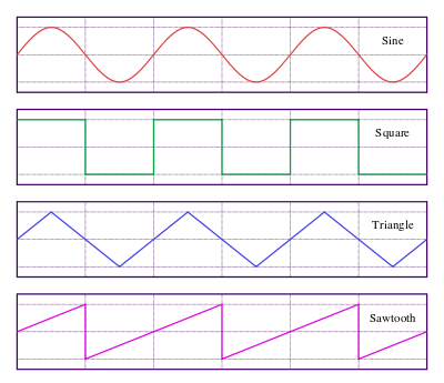
【Sine Wave】
 ,
,
【Square Wave】
 ,
,
【Triangle Wave】
 ,
, 
【Sawtouth Wave】
 ,
,
,此處
 是『時間』,
是『頻率』,
 是『振幅』,
 是
是  的『分數部份』 Fractional part。
── 如果命運果真有規劃局;事物就定能分好類嗎??──
─── 引自《【Sonic π】電聲學之電路學《一》下》
貫通之後,或將能對 Miller Puckette 書中所言︰
1.2 Units of Amplitude
Two amplitudes are often better compared using their ratio than their difference. Saying that one signal’s amplitude is greater than another’s by a factor of two might be more informative than saying it is greater by 30 millivolts. This is true for any measure of amplitude (RMS or peak, for instance). To facilitate comparisons, we often express amplitudes in logarithmic units called decibels. If a is the amplitude of a signal (either peak or RMS), then we can define the
decibel (dB) level d as:
where a0 is a reference amplitude.
………
有更深入之理解耶!?