雖然不知道『聲波』振動與傳播的物理,並不妨礙 Miller Puckette 先生書中文章之應用。然而若能知道那些原理,或許可以深化理解 ,不只是『知其然』,進而能知『所以然』的吧!所以此處先列出一些與之相關文本系列之首篇,方便讀者參考︰
以期在運用科技之時,還能欣賞自然耶!!
比方說 Miller Puckette 在 1.6 節文中,用著簡易的數學來談『訊號疊加』現象,
1.6 Superposing Signals
If a signal x[n] has a peak or RMS amplitude A (in some fixed window), then the scaled signal k · x[n] (where k ≥ 0) has amplitude kA. The mean power of the scaled signal changes by a factor of k 2 . The situation gets more complicated when two different signals are added together; just knowing the amplitudes of the two does not suffice to know the amplitude of the sum. The two amplitude measures do at least obey triangle inequalities; for any two signals x[n] and y[n],


If we fix a window from M to N + M − 1 as usual, we can write out the mean power of the sum of two signals:

where we have introduced the covariance of two signals:

The covariance may be positive, zero, or negative. Over a sufficiently large window, the covariance of two sinusoids with different frequencies is negligible compared to the mean power. Two signals which have no covariance are called uncorrelated (the correlation is the covariance normalized to lie between -1 and 1). In general, for two uncorrelated signals, the power of the sum is the sum of the powers:

Put in terms of amplitude, this becomes:

This is the familiar Pythagorean relation. So uncorrelated signals can be thought of as vectors at right angles to each other; positively correlated ones as having an acute angle between them, and negatively correlated as having an obtuse angle between them.
For example, if two uncorrelated signals both have RMS amplitude a, the sum will have RMS amplitude  . On the other hand if the two signals happen to be equal—the most correlated possible—the sum will have amplitude 2a, which is the maximum allowed by the triangle inequality.
………
引出『不相關』 uncorrelated 訊號間有直角三角形『畢氏關係』。說明了頻率不同之『正弦波』 sinusoids 通常『不相關』 。假使此時補之以《【Sonic π】聲波之傳播原理︰原理篇《四下》》文本所講的『駐波』,這也是許多『樂器』的發聲原理︰

駐波形成
在一輛長列『左行』的火車上有一個很長的『水槽』,上有一向右的『行進波』

,假使向左的火車與向右之水波速度相同,那麼一位站在月台的『觀察者』 將如何描述那個『行進波』的呢?
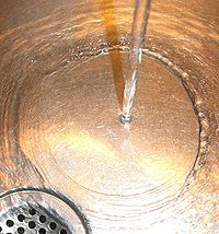
如果觀察水由水龍頭注入水槽的現象,由於水在到達槽底前的流速『較快』,然而到達槽底後水的流速突然的『變慢』,因此會發生『水躍』Hydraulic jump 的現象,此時水之部份動能將轉換為位能,故而在槽底的液面形成『駐波』。這個現象在『河水』的『流速』突然『由快變慢』時也可能發生,因而有人能在『河裡衝浪』,他正站在『駐波』之上!!
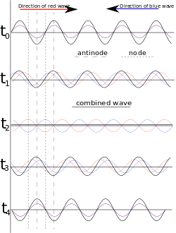
那什麼是『駐波』的呢?比方說一個『不動的』stationary 介質中,向左的波  與向右的波
與向右的波  疊加後的『合成波』
 ,在『特定』的『邊界條件』下,被『侷限』在一定『空間區域』內無法前進,因此稱為『駐波』。由於駐波不能傳播能量,它的能量將『儲存』在那個空間區域裡。駐波所在區域,『振幅為零』的點稱為『節點』或『波節』Node ,『振幅最大』的點位於兩『節點』之間,通常叫做『腹點』或『波腹』Antinode。
![]()

一根長度  震盪的弦上,一個向右的簡諧波
  ,由於弦的兩頭固定,那個波在右端點也只能『反射』回來,形成了
  ,此時合成波
  是
是

,可用三角恆等式簡化為

。此時『時間項』與『空間項』分離,形成『駐波』。在  時,
時, ,此處
,此處  是整數,這就是『節點』;當
  時
時  ,也就是『腹點』。當然波長
  就得滿足
就得滿足  的邊界條件。
─── 琴弦擇音而振, 苟非知音焉得共鳴。───
───
當更能了解那些滿足 『波長』關係的『頻率』構成了那根『弦』的『泛音』。不同『音色』的『弦』正因此『泛音』頻譜不同而出色。或也將知這也是『正交函數族』 Orthogonal functions 的發展以及『傅立葉級數』之歷史濫觴乎︰
Hilbert space interpretation
In the language of Hilbert spaces, the set of functions { ; n ∈ Z} is an orthonormal basis for the space L2([−π, π]) of square-integrable functions of [−π, π]. This space is actually a Hilbert space with an inner product given for any two elements f and g by

The basic Fourier series result for Hilbert spaces can be written as

- This corresponds exactly to the complex exponential formulation given above. The version with sines and cosines is also justified with the Hilbert space interpretation. Indeed, the sines and cosines form an orthogonal set:

- Sines and cosines form an orthonormal set, as illustrated above. The integral of sine, cosine and their product is zero (green and red areas are equal, and cancel out) when m, n or the functions are different, and pi only if m and n are equal, and the function used is the same.
-
(where δmn is the Kronecker delta), and
furthermore, the sines and cosines are orthogonal to the constant function 1. An orthonormal basis for L2([−π,π]) consisting of real functions is formed by the functions 1 and √2 cos(nx), √2 sin(nx) with n = 1, 2,… The density of their span is a consequence of the Stone–Weierstrass theorem, but follows also from the properties of classical kernels like the Fejér kernel.


───
若非如此,樂器將如何和鳴共奏呢?或終可聞箱子天籟之聲的耶 ??!!