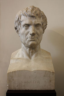
即使以相同的『數學方法』,因為談論不同的事,有時還是得腦筋『急轉彎』。這個腦筋『急轉彎』的由來,也許是因為得用『非常不同』的觀點來考察事物。突然發現某種不期而遇之『共通處』。若問笛卡爾如何想出『解析幾何』,使得幾何得以用『座標系』與『座標』來處理?雖說不得而知,但是這套數學『思維方法』構成了牛頓力學的骨幹。就像問著『約瑟夫‧傅立葉』 Joseph Fourier 為什麼會將函數用『正弦級數』來作展開??難道是受到笛卡爾的啟發!或是牛頓的影響!!可能很難定論。此處只能借著科學史上的一個小故事來暗示那種概念間冥冥的『聯繫』︰
電阻的單位是『歐姆』
傅立葉分析
數學上最美麗的樂章


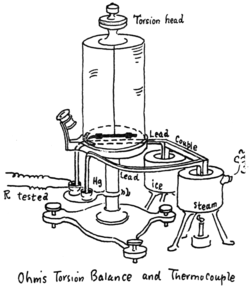
一八二五年德國物理學家蓋歐格‧西蒙‧歐姆 Georg Simon Ohm 是一位優秀的實驗者,很會設計與製造實驗設備,又具有良好的數學素養和嚴謹的處事態度。他使用伏打電堆為電源,繼而用安裝於扭秤 torsion balance 的磁針來測量電流產生的磁力。因為載流導線的電流所產生的磁場與電流成正比,所以只要測量在載流導線附近的磁針所感受到的磁力,就可以度量電流的大小。 他將電流通過不同長度的受測電線;由於長度的不同,電流也就不同。並且基於實驗結果推導出了兩者之間的數學關係式︰

其中, 是受測電線造成的電流差值,
 是跟實驗參數有關的係數,
 是受測電線的長度,
 是跟固定長度的載流導線有關的常數。不久之後,歐姆便發覺了這個關係式可能是不正確的。
法國數學家與物理學家約瑟夫‧傅立葉男爵 Joseph Fourier 以所提出的『傅立葉級數』稱名於世,對於任何一個周期為  的函數
的函數  ,都可以用『無窮級數』表示為

,式中係數  可以依下式來計算

。此處  ,而且
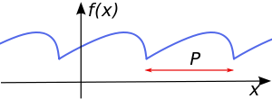
,而且  是基本周期為 的三角『正、餘弦』函數,這就是周期訊號 的『諧波分析』。當
  時,
時, 係數稱之為『直流分量』,就是訊號 在整個周期的平均值。當
  時,
時, 係數是『一次諧波』頻率,隨著
  的值,而有『二次諧波』,『三次諧波』等等。並且將之應用於『熱傳導理論』與『振動理論』;據聞他也是『溫室效應』的發現者。一八二二年傅立葉發表了《熱的解析理論》 Théorie analytique de la chaleur)。依據『牛頓冷卻定律』假設了︰兩相鄰分子的熱流與其間微小的溫度差成正比。
受到傅立葉對熱傳導規律研究的啟發,歐姆認為『電流現象』與『熱傳導』相似,便猜想導線中兩點之間的電流也正比於這兩點間的某種驅動力 ── 即現在所說的『電動勢』 ──。由於當時『伏打電堆』所產生的電流並不穩定,據聞歐姆採納了《物理與化學年鑑》的總編輯約翰‧波根多夫 Johann poggendorff 的建議,改用『熱電偶』為電源。雖然『鉍和銅』所作的『溫差電池』保證了電流的穩定性。然而卻產生了測量『電流太小』的難題。歐姆先是利用『電流』的『熱效應』,想藉著『熱脹冷縮』的方法來測量電流大小,但是量測的結果並『不精確』,後來他把奧斯特『電流磁效應』的發現和『庫侖扭秤』巧妙的結合起來設計了一個『電流扭秤』︰讓導線和連接的磁針平行放置,當導線中通過電流時,磁針的偏轉角與導線中的電流成正比,這就代表了電流的大小。
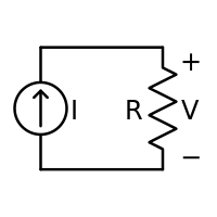
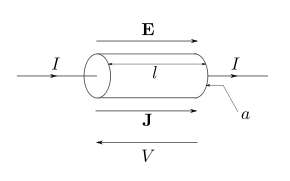
一八二六年歐姆所發表兩篇重要論文中,建立了『電傳導』的『數學模型』和『表達式』。著名的『歐姆定律』發表於一八二七年的《直流電路的數學研究》 Die galvanische Kette, mathematisch bearbeitet 一書中,提出了『電路分析』中『電流』、『電壓』與『電阻』之間的基本關係
 。
。
─── 引自《【Sonic π】電聲學導引《七》》
或許能說明『正交函數族』之概念,並非一蹴而成的,所謂『正交 』也不可講成『畢氏定理』自然的擴張。雖然說這些『象徵』表達概念可能的深層『融會』,提示讀者進入的門徑。究其實,依舊是例說寓言罷了。
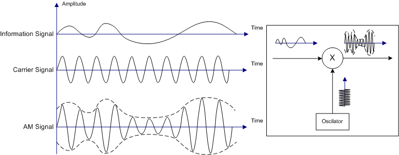
就像『振幅調變』  之『頻譜』,可以用『頻譜摺積』來計算,然而什麼是『摺積』呢?
Convolution
In mathematics and, in particular, functional analysis, convolution is a mathematical operation on two functions f and g, producing a third function that is typically viewed as a modified version of one of the original functions, giving the area overlap between the two functions as a function of the amount that one of the original functions is translated. Convolution is similar to cross-correlation. It has applications that include probability, statistics, computer vision, natural language processing, image and signal processing, engineering, and differential equations.
The convolution can be defined for functions on groups other than Euclidean space. For example, periodic functions, such as the discrete-time Fourier transform, can be defined on a circle and convolved by periodic convolution. (See row 10 at DTFT#Properties.) A discrete convolution can be defined for functions on the set of integers. Generalizations of convolution have applications in the field of numerical analysis and numerical linear algebra, and in the design and implementation of finite impulse response filters in signal processing.
Computing the inverse of the convolution operation is known as deconvolution.
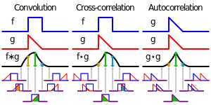
Visual comparison of convolution, cross-correlation and autocorrelation.
摺積
在泛函分析中,捲積、疊積、摺積或旋積,是通過兩個函數f和g生成第三個函數的一種數學算子,表徵函數f與經過翻轉和平移的g的重疊部分的面積。如果將參加摺積的一個函數看作區間的指示函數,摺積還可以被看作是「滑動平均」的推廣。
圖示兩個方形脈衝波的捲積。其中函數”g”首先對 反射,接著平移”t”,成為
 。那麼重疊部份的面積就相當於”t”處的捲積,其中橫坐標代表待積變量
 以及新函數
以及新函數 的自變量”t”。
圖示方形脈衝波和指數衰退的脈衝波的捲積(後者可能出現於RC電路中),同樣地重疊部份面積就相當於”t”處的捲積。注意到因為”g”是對稱的,所以在這兩張圖中,反射並不會改變它的形狀。
簡單介紹
摺積是分析數學中一種重要的運算。設: ,
, 是
是 上的兩個可積函數,作積分:

可以證明,關於幾乎所有的 ,上述積分是存在的。這樣,隨著
 的不同取值,這個積分就定義了一個新函數
 ,稱為函數
,稱為函數 與
與 的摺積,記為
 。我們可以輕易驗證:
 ,並且
,並且 仍為可積函數。這就是說,把摺積代替乘法,
 空間是一個代數,甚至是巴拿赫代數。雖然這裡為了方便我們假設
  ,不過捲積只是運算符號,理論上並不需要對函數
  有特別的限制,雖然常常要求 至少是可測函數(measurable function)(如果不是可測函數的話,積分可能根本沒有意義),至於生成的卷積函數性質會在運算之後討論。
摺積與傅立葉變換有著密切的關係。例如兩函數的傅立葉變換的乘積等於它們摺積後的傅立葉變換,利用此一性質,能簡化傅立葉分析中的許多問題。
由摺積得到的函數 一般要比和都光滑。特別當為具有緊支集的光滑函數,為局部可積時,它們的摺積也是光滑函數。利用這一性質,對於任意的可積函數,都可以簡單地構造出一列逼近於的光滑函數列
 ,這種方法稱為函數的光滑化或正則化。
摺積的概念還可以推廣到數列、測度以及廣義函數上去。
The convolution theorem and its applications
What is a convolution?
One of the most important concepts in Fourier theory, and in crystallography, is that of a convolution. Convolutions arise in many guises, as will be shown below. Because of a mathematical property of the Fourier transform, referred to as the convolution theorem, it is convenient to carry out calculations involving convolutions.
But first we should define what a convolution is. Understanding the concept of a convolution operation is more important than understanding a proof of the convolution theorem, but it may be more difficult!
Mathematically, a convolution is defined as the integral over all space of one function at x times another function at u-x. The integration is taken over the variable x (which may be a 1D or 3D variable), typically from minus infinity to infinity over all the dimensions. So the convolution is a function of a new variable u, as shown in the following equations. The cross in a circle is used to indicate the convolution operation.
Note that it doesn’t matter which function you take first, i.e. the convolution operation is commutative. We’ll prove that below, but you should think about this in terms of the illustration below. This illustration shows how you can think about the convolution, as giving a weighted sum of shifted copies of one function: the weights are given by the function value of the second function at the shift vector. The top pair of graphs shows the original functions. The next three pairs of graphs show (on the left) the function g shifted by various values of x and, on the right, that shifted function g multiplied by f at the value of x.
The bottom pair of graphs shows, on the left, the superposition of several weighted and shifted copies of g and, on the right, the integral (i.e. the sum of all the weighted, shifted copies of g). You can see that the biggest contribution comes from the copy shifted by 3, i.e. the position of the peak of f.
If one of the functions is unimodal (has one peak), as in this illustration, the other function will be shifted by a vector equivalent to the position of the peak, and smeared out by an amount that depends on how sharp the peak is. But alternatively we could switch the roles of the two functions, and we would see that the bimodal function g has doubled the peaks of the unimodal function f.
───
它是否有所謂傳統『乘法類似物』的耶!!或者『類比推理』只該看成是『發現』的邏輯乎??


 .
. is an
is an  is a representation of a 1-periodic function.
 為『周期』的函數,自然也以
  為周期【※
為周期【※  非零正整數】,所以實數周期函數才會有最小周期值。
 以
以  為周期,
為周期,  以
以  為周期,假使
  的比值是個『有理數』,可以用『最簡分數』表示成
  。也就是說
。也就是說 
 的周期。然而周期不必是『有理數』,周期的『比值』當然也未必是『有理數』,因此
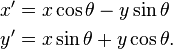
 三個參數?即使在思考過
  是此『底』之『高』,
  是此『高』距與此『底』一端的距離。我們深信這就『確定』了那個三角形。然而若再問︰如果此三角形的三個頂點用更一般的
  、
、  、
、  來表達 ,如是分明有六個參數。那麼這兩種『表述』當真是一樣的嗎?設想你在桌面上『移動』一個三角形,從此『位置』此『方位』到達彼『位置』彼『方位』,你會認為這個三角形『改變』了嗎??假使『直覺』以為『不變』,這個三角形就必得有使之『不變』的『因由』,這個『因由』不必『參照』解析幾何的『座標』而確立 。或可說它就是歐式幾何一個三角形的『定義』內涵而已。如此而言,一個『確定』的三角形,可由它的三個『邊長』來『確立』,所以六個參數補之以三個確定之邊長關係,豈非還是三個參數的耶??

 .
.
 and
and  have the same magnitude and are separated by an angle

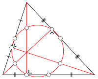
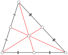
 、
、 、
、 為三邊的中點,
 、
、 、
、 為垂足,
為垂足, 、
、 、
、 為和頂點到垂心的三條線段的中點。
 、
、 (
(
 、
、 (SAS相似)
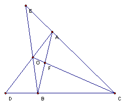
 ,可得出四邊形
 是
是 也是矩形(
也是矩形( 共圓)
共圓) ,因此可知
,因此可知

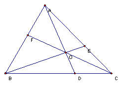
 的塞瓦線段AD、BE、CF通過同一點O,則


 決定一條線,這線的方程式可以寫成
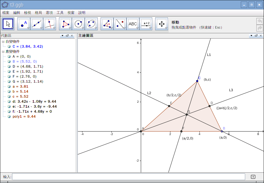
 ,不失一般性,假設這三個頂點座標是
  ,那麼
,那麼


 ,
, ,和
,和 ,那麼幾何中心位於:


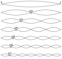

 ,與『調和級數』
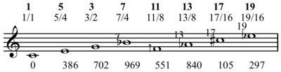
  的『調和』之名源於『樂理』中的『泛音』 overtone 和『泛音列』 harmonic series。
 是一個『調和序列』的第
  就是
就是  ,所以
,所以  。於是『調和序列』中任意連續的三個數
  『全部』都構成了『調和平均數』之『關係』
  。因此這就是『為什麼』那個『調和序列』會被稱之為『調和』的了。現實裡,大概也只有大自然中,那不期而遇的『山光水影』之『漸層』 的『美』,方能夠與之『匹配』的吧!!
 .
. ,
,
![= [1 + m(t)]\cdot c(t) \,](https://upload.wikimedia.org/math/a/2/c/a2c3cc7febcb13a24495274319bd6730.png)
![= [1 + M\cdot \cos(2 \pi f_m t + \phi)] \cdot A \cdot \sin(2 \pi f_c t)](https://upload.wikimedia.org/math/3/d/9/3d96e992b9e94194dace10fe42fe45da.png)
![y(t) = A\cdot \sin(2 \pi f_c t) + \begin{matrix}\frac{AM}{2} \end{matrix} \left[\sin(2 \pi (f_c + f_m) t + \phi) + \sin(2 \pi (f_c - f_m) t - \phi)\right].\,](https://upload.wikimedia.org/math/8/a/a/8aac05f9aceaf90faadc45f830b52dd9.png)