再別康橋‧徐志摩

輕輕的我走了，
正如我輕輕的來；
我輕輕的招手，
作別西天的雲彩。

那河畔的金柳 是夕陽中的新娘；
波光裡的艷影，
在我的心頭蕩漾。

軟泥上的青荇 油油的在水底招搖：
在康河的柔波裡 我甘心做一條水草！
那榆蔭下的一潭 不是清泉，
是天上虹 揉碎在浮藻間，
沉澱著彩虹似的夢。

尋夢？
撐一支長篙 向青草更青處漫溯，
滿載一船星輝，
在星輝斑爛裡放歌。

但我不能放歌，
悄悄是別離的笙簫；
夏蟲也為我沉默，
沉默是今晚的康橋！

悄悄的我走了，
正如我悄悄的來；
我揮一揮衣袖，
不帶走一片雲彩。

 

人們見不著『徐志摩的康橋』並非因為『目盲』，只是無法用他之眼光去看？

人們聽不明『巴斯卡的論證』

過去法國的哲學家 Blaise Pascal 寫過一本《沉思錄》，這本書裡頭有一個很有意思的論證︰

無神論者之不幸

如果你信仰上帝，但是祂不存在，你沒有損失；
假使你不信仰上帝，然而祂卻存在，你會下地獄；
權衡利弊，你還是信仰上帝的好。

『思想的蘆葦』之說法果真不同凡響，其後有人推廣了巴斯卡的論證及於『諸神』，所謂『多多益善』，誰又想少了一個『保佑』！同時又身為科學家和數學家的他，他心中『懷疑』的精神與心靈『信仰』的熱忱，似乎並不矛盾彷彿完美結合。這難道是奇怪的事嗎？由於科學研究的是『有了的』世界，尚未知或終不能研究『從無到有』的『大創造』。因此許多的科學家擁有自己的『信仰』，那又有什麼好奇怪的呢？畢竟問著生命的『來之何處』和『去向何方』？或許只是人想知道『我是誰』？也許人的一生總該有如此『自問』的時候吧？？

─── 摘自《目盲與耳聾》

 

豈是由於『耳聾』，或許他早已透視『文藝復興』的哩？

窮百代之追尋，留有遺產乎？？

History

The first geometrical properties of a projective nature were discovered during the 3rd century by Pappus of Alexandria.^[3] Filippo Brunelleschi (1404–1472) started investigating the geometry of perspective during 1425^[10] (see the history of perspective for a more thorough discussion of the work in the fine arts that motivated much of the development of projective geometry). Johannes Kepler (1571–1630) and Gérard Desargues (1591–1661) independently developed the concept of the “point at infinity”.^[11] Desargues developed an alternative way of constructing perspective drawings by generalizing the use of vanishing points to include the case when these are infinitely far away. He made Euclidean geometry, where parallel lines are truly parallel, into a special case of an all-encompassing geometric system. Desargues’s study on conic sections drew the attention of 16-year-old Blaise Pascal and helped him formulate Pascal’s theorem. The works of Gaspard Monge at the end of 18th and beginning of 19th century were important for the subsequent development of projective geometry. The work of Desargues was ignored until Michel Chasles chanced upon a handwritten copy during 1845. Meanwhile, Jean-Victor Poncelet had published the foundational treatise on projective geometry during 1822. Poncelet separated the projective properties of objects in individual class and establishing a relationship between metric and projective properties. The non-Euclidean geometries discovered soon thereafter were eventually demonstrated to have models, such as the Klein model of hyperbolic space, relating to projective geometry.

This early 19th century projective geometry was intermediate from analytic geometry to algebraic geometry. When treated in terms of homogeneous coordinates, projective geometry seems like an extension or technical improvement of the use of coordinates to reduce geometric problems to algebra, an extension reducing the number of special cases. The detailed study of quadrics and the “line geometry” of Julius Plücker still form a rich set of examples for geometers working with more general concepts.

The work of Poncelet, Jakob Steiner and others was not intended to extend analytic geometry. Techniques were supposed to be synthetic: in effect projective space as now understood was to be introduced axiomatically. As a result, reformulating early work in projective geometry so that it satisfies current standards of rigor can be somewhat difficult. Even in the case of the projective plane alone, the axiomatic approach can result in models not describable via linear algebra.

This period in geometry was overtaken by research on the general algebraic curve by Clebsch, Riemann, Max Noether and others, which stretched existing techniques, and then by invariant theory. Towards the end of the century, the Italian school of algebraic geometry (Enriques, Segre, Severi) broke out of the traditional subject matter into an area demanding deeper techniques.

During the later part of the 19th century, the detailed study of projective geometry became less fashionable, although the literature is voluminous. Some important work was done in enumerative geometry in particular, by Schubert, that is now considered as anticipating the theory of Chern classes, taken as representing the algebraic topology of Grassmannians.

Paul Dirac studied projective geometry and used it as a basis for developing his concepts of quantum mechanics, although his published results were always in algebraic form. See a blog article referring to an article and a book on this subject, also to a talk Dirac gave to a general audience during 1972 in Boston about projective geometry, without specifics as to its application in his physics.

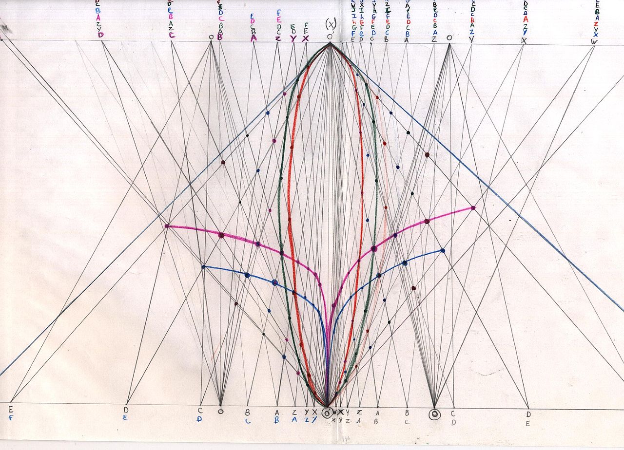
Growth measure and the polar vortices. Based on the work of Lawrence Edwards

 

若問幾眼注目才能看清！！

Three-point perspective

Three-point perspective is often used for buildings seen from above (or below). In addition to the two vanishing points from before, one for each wall, there is now one for how the vertical lines of the walls recede. For an object seen from above, this third vanishing point is below the ground. For an object seen from below, as when the viewer looks up at a tall building, the third vanishing point is high in space.

Three-point perspective exists when the perspective is a view of a Cartesian scene where the picture plane is not parallel to any of the scene’s three axes. Each of the three vanishing points corresponds with one of the three axes of the scene. One, two and three-point perspectives appear to embody different forms of calculated perspective, and are generated by different methods. Mathematically, however, all three are identical; the difference is merely in the relative orientation of the rectilinear scene to the viewer.

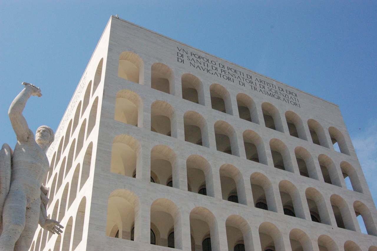
The Palazzo del Lavoro in Mussolini’s Esposizione Universale Roma complex, photographed in 3-point perspective. All three axes are oblique to the picture plane; the three vanishing points are at the zenith, and on the horizon to the right and left.

 

 多少套餐方可養分無虞？？

Epipolar Geometry

 

答案啊！答案？在茫茫的風裡！！？？