若問薄透鏡之理想性何在?又為什麼會成為理論法寶的呢!得先從兩個曲面  、
、  的折射推導出薄透鏡

以及造透鏡者公式
![\Phi (R_1, R_2) = \frac{1}{f} = (n-1) \left[ \frac{1}{R_1} - \frac{1}{R_2} \right]](https://www.freesandal.org/wp-content/ql-cache/quicklatex.com-c786934eb649a711256ab841df2bc7f1_l3.png "Rendered by QuickLaTeX.com") 講起。
講起。
因為  的反對稱性︰

當 薄透鏡由  反轉成
反轉成  時,凹面將變凸面、凸面將變凹面,此時
  、 依約定之符號正負慣例,皆需變號,反倒使薄透鏡維持反轉不變性。故知薄透鏡前、後焦距一樣就是焦距
  。事實上由於薄透鏡的特殊矩陣形制,兩個緊貼之薄透鏡組合還滿足交換律的哩︰

其次薄透鏡的
端點面 = 主平面 = 節點面

,此處  是物距,
是物距,  是像距。
是像距。
在此成像條件下,總合矩陣可表示成︰
 。
。
也就是說總合矩陣的 參數等於
參數等於  。
。
若以放大率  之定義,可將之改寫為︰
 。
。
此處負號是說︰假如 是正的,將聚焦產生倒立之實像也。
雖然沿著光徑走,經過一個透鏡,才能到下個透鏡,光子不必知有幾村幾店,不過是走過這村到那店,因此
物成像,像做物。
依序聚散罷了,講其是否能『串接成像』而已︰

不過符號眾多,代數運算麻煩,而且易為虛實正負物距像距鬧的個頭昏腦轉。即使知兩個一般光學矩陣

就可代表『人眼見物』或『鏡頭攝物』,卻難了那個 ABCD 之光學矩陣實為人眼或鏡頭所設計出的觀物設備矣。
因此通熟薄透鏡的基本成像法則
之作用︰物已成像,像即是物。實 是關鍵處也。若說起初物在透鏡之外, 則  ,但如成像落在下個薄透鏡之內,那麼
  ,於是正負與虛實之理相互爭勝, 用前一薄透鏡定之哉 ?或以後一薄透鏡定之哉!還是由薄透鏡組合定之哉??!!設若將此議論用之於像,豈不依然焉!!??奈何懷疑人眼或鏡頭只見虛像或實像呢★?倘已成像,就 是看到像了吧,又怎能不實的哩 。此時所謂設備之有無,難到不祇是為方不方便觀物的嗎☆!
── 摘自《光的世界︰【□○閱讀】樹莓派近攝鏡‧下‧答之起》
難到『幾何光學三條線』不座落在同一平面上嗎?莫非『成像法則 』不是用『線狀物』描述耶??靜思光學系統通常有『光軸旋轉』『對稱性』,可得『沙漏』之意象乎!

安布羅喬洛倫采蒂的作品: Allegory of Good Government, 1338年
或許『沙漏』不止是度量『時間』,還潛藏著『針孔相機模型』的『奧秘』!!
熟悉的事物往往容易疑惑,然而意料之外的難處卻能加深理解◎
試讀『一維投影』的若干文摘︰
Projective line
In mathematics, a projective line is, roughly speaking, the extension of a usual line by a point called a point at infinity. The statement and the proof of many theorems of geometry are simplified by the resultant elimination of special cases; for example, two distinct projective lines in a projective plane meet in exactly one point (there is no “parallel” case).
There are many equivalent ways to formally define a projective line; one of the most common is to define a projective line over a field K, commonly denoted P1(K), as the set of one-dimensional subspaces of a two-dimensional K–vector space. This definition is a special instance of the general definition of a projective space.
Homogeneous coordinates
An arbitrary point in the projective line P1(K) may be represented by an equivalence class of homogeneous coordinates, which take the form of a pair
![[x_1 : x_2]](https://wikimedia.org/api/rest_v1/media/math/render/svg/09404e16ef9ccccd05414dabeedac84b306fe9e4)
of elements of K that are not both zero. Two such pairs are equivalent if they differ by an overall nonzero factor λ:
![[x_{1}:x_{2}]\sim [\lambda x_{1}:\lambda x_{2}].](https://wikimedia.org/api/rest_v1/media/math/render/svg/0e149dfacd2fd2bfcc157bc3da4e654227498373)
Line extended by a point at infinity
The projective line may be identified with the line K extended by a point at infinity. More precisely, the line K may be identified with the subset of P1(K) given by
![\left\{[x : 1] \in \mathbf P^1(K) \mid x \in K\right\}.](https://wikimedia.org/api/rest_v1/media/math/render/svg/086c5d6b3f2d24eccfa35f0847c01d70c75b8c57)
This subset covers all points in P1(K) except one, which is called the point at infinity:
![\infty = [1 : 0].](https://wikimedia.org/api/rest_v1/media/math/render/svg/54a6746d720a3849c5aeeeb5b0cb7fb0f12eac33)
This allows to extend the arithmetic on K to P1(K) by the formulas


Translating this arithmetic in term of homogeneous coordinates gives, when [0 : 0] does not occur:
![[x_1 : x_2] + [y_1 : y_2] = [x_1 y_2 + y_1 x_2 : x_2 y_2],](https://wikimedia.org/api/rest_v1/media/math/render/svg/94336d2523cfacf85e317a6516fe913cf0e030fd)
![[x_1 : x_2] \cdot [y_1 : y_2] = [x_1 y_1 : x_2 y_2],](https://wikimedia.org/api/rest_v1/media/math/render/svg/94fa88c74d83459420ba532b4549908fd14cbab9)
![[x_1 : x_2]^{-1} = [x_2 : x_1].](https://wikimedia.org/api/rest_v1/media/math/render/svg/c8afadaa9e638cbce6c51e27ae575b77755bc3cc)
Examples
Real projective line
The projective line over the real numbers is called the real projective line. It may also be thought of as the line K together with an idealised point at infinity ∞ ; the point connects to both ends of K creating a closed loop or topological circle.
An example is obtained by projecting points in R2 onto the unit circle and then identifying diametrically opposite points. In terms of group theory we can take the quotient by the subgroup {1, −1}.
Compare the extended real number line, which distinguishes ∞ and −∞.
Homography
In projective geometry, a homography is an isomorphism of projective spaces, induced by an isomorphism of the vector spaces from which the projective spaces derive.[1] It is a bijection that maps lines to lines, and thus a collineation. In general, some collineations are not homographies, but the fundamental theorem of projective geometry asserts that is not so in the case of real projective spaces of dimension at least two. Synonyms include projectivity, projective transformation, and projective collineation.
Historically, homographies (and projective spaces) have been introduced to study perspective and projections in Euclidean geometry, and the term homography, which, etymologically, roughly means “similar drawing” date from this time. At the end of the 19th century, formal definitions of projective spaces were introduced, which differed from extending Euclidean or affine spaces by adding points at infinity. The term “projective transformation” originated in these abstract constructions. These constructions divide into two classes that have been shown to be equivalent. A projective space may be constructed as the set of the lines of a vector space over a given field (the above definition is based on this version); this construction facilitates the definition of projective coordinates and allows using the tools of linear algebra for the study of homographies. The alternative approach consists in defining the projective space through a set of axioms, which do not involve explicitly any field (incidence geometry, see also synthetic geometry); in this context, collineations are easier to define than homographies, and homographies are defined as specific collineations, thus called “projective collineations”.
For sake of simplicity, unless otherwise stated, the projective spaces considered in this article are supposed to be defined over a (commutative) field. Equivalently Pappus’s hexagon theorem and Desargues’ theorem are supposed to be true. A large part of the results remain true, or may be generalized to projective geometries for which these theorems do not hold.
Geometric motivation
Historically, the concept of homography had been introduced to understand, explain and study visual perspective, and, specifically, the difference in appearance of two plane objects viewed from different points of view.
In the Euclidean space of dimension 3, a central projection from a point O (the center) onto a plane P that does not contain O is the mapping that sends a point A to the intersection (if it exists) of the line OA and the plane P. The projection is not defined if the point A belongs to the plane passing through O and parallel to P. The notion of projective space was originally introduced by extending the Euclidean space, that is, by adding points at infinity to it, in order to define the projection for every point except O.
Given another plane Q, which does not contain O, the restriction to Q of the above projection is called a perspectivity.
With these definitions, a perspectivity is only a partial function, but it becomes a bijection if extended to projective spaces. Therefore, this notion is normally defined for projective spaces. The notion is also easily generalized to projective spaces of any dimension, over any field, in the following way: Given two projective spaces P and Q of dimension n, a perspectivity is a bijection from P to Q that may be obtained by embedding P and Q in a projective space R of dimension n + 1 and restricting to P a central projection onto Q.
If f is a perspectivity from P to Q, and g a perspectivity from Q to P, with a different center, then g ⋅ f is a homography from P to itself, which is called a central collineation, when the dimension of P is at least two. (see § Central collineation below and Perspectivity § Perspective collineations).
Originally, a homography was defined as the composition of a finite number of perspectivities.[2] It is a part of the fundamental theorem of projective geometry (see below) that this definition coincides with the more algebraic definition sketched in the introduction and detailed below.
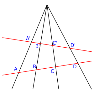
Points A, B, C, D and A′, B′, C′, D′ are related by a perspectivity, which is a projective transformation.
Perspectivity
In geometry and in its applications to drawing, a perspectivity is the formation of an image in a picture plane of a scene viewed from a fixed point.
Graphics
The science of graphical perspective uses perspectivities to make realistic images in proper proportion. According to Kirsti Andersen, the first author to describe perspectivity was Leon Alberti in his De Pictura (1435).[1] In English, Brook Taylor presented his Linear Perspective in 1715, where he explained “Perspective is the Art of drawing on a Plane the Appearances of any Figures, by the Rules of Geometry”.[2] In a second book, New Principles of Linear Perspective (1719), Taylor wrote
- When Lines drawn according to a certain Law from the several Parts of any Figure, cut a Plane, and by that Cutting or Intersection describe a figure on that Plane, that Figure so described is called the Projection of the other Figure. The Lines producing that Projection, taken all together, are called the System of Rays. And when those Rays all pass thro’ one and same Point, they are called the Cone of Rays. And when that Point is consider’d as the Eye of a Spectator, that System of Rays is called the Optic Cone[3]
Projective geometry
In projective geometry the points of a line are called a projective range, and the set of lines in a plane on a point is called a pencil.
Given two lines 


![f_P \colon [\ell] \mapsto [m]](https://wikimedia.org/api/rest_v1/media/math/render/svg/0e04d1a74b6fa3b728499e363eb7ac0b25c08393)

![f_P (f_P (X)) = X \text{ for all }X \in [\ell]](https://wikimedia.org/api/rest_v1/media/math/render/svg/8b1a2bb9dee33511a3eea59395c7d55942a4275b)
The existence of a perspectivity means that corresponding points are in perspective. The dual concept, axial perspectivity, is the correspondence between the lines of two pencils determined by a projective range.
Projectivity
The composition of two perspectivities is, in general, not a perspectivity. A perspectivity or a composition of two or more perspectivities is called a projectivity (projective transformation, projective collineation and homography are synonyms).
There are several results concerning projectivities and perspectivities which hold in any pappian projective plane:[6]
Theorem: Any projectivity between two distinct projective ranges can be written as the composition of no more than two perspectivities.
Theorem: Any projectivity from a projective range to itself can be written as the composition of three perspectivities.
Theorem: A projectivity between two distinct projective ranges which fixes a point is a perspectivity.
A perspectivity:

默想平面國 Flatland 之藝術家會怎麼認識它呢☆
The Real Projective Line
J.C. Álvarez Paiva
In this chapter we study the action of the projective group on the real projective line.
- Anything preceded by a * may be left for a second reading.
- Next to the exercises there is a two-digit number in parentheses which describes its degree of difficulty. The simplest exercises are identified by a (00), while the hardest — those that could take you a week of intensive brain work — are identified by a (50).
- Basic definitions
- The fundamental theorems
- Harmonic quadruples and von Staudt’s theorem
- Bibliography
- About this document …
Juan Carlos Alvarez 2000-10-27
Basic definitions
 is the set of all lines in
  passing through the origin.
Note that if  and
and  are two nonzero vectors lying on the same line through the origin, then they are multiples of each other. This remark allows us to redefine
  as the quotient of
  by the equivalence relation
  (or
(or  ) if and are multiples of each other.
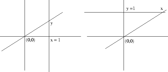
Exercise 1.6 (00) Let  be the slope of the line
  passing through the origin and let

be an invertible matrix. Verify that the slope of the line  equals
  .
.
This exercise tells us that in suitable coordinates projective transformations have the form  .
.
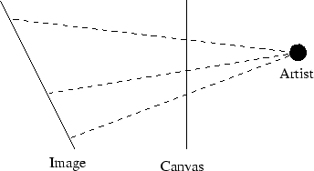
As explained in [2], projective geometry arose from the artists’ needs to represent the three-dimensional world on a two-dimensional canvas. An artist in Flatland just has to worry about representing a two-dimensional world on a one-dimensional canvas. The figure below shows a Flatland artist copying a one-dimensional image onto a canvas. Notice how distances are distorted.
This type of correspondence between the points in two lines is called a perspective.