《繚綾》 唐‧白居易

繚綾繚綾何所似，不似羅綃與紈綺。
應似天台山上月明前，四十五尺瀑布泉。
中有文章又奇絕，地鋪白煙花簇雪。
織者何人衣者誰，越溪寒女漢宮姬。
去年中使宣口敕，天上取樣人間織。
織爲雲外秋雁行，染作江南春水色。
廣裁衫袖長制裙，金鬥熨波刀翦紋。
異彩奇文相隱映，轉側看花花不定。
昭陽舞人恩正深，春衣一對直千金。
汗沾粉污不再著，曳土蹋泥無惜心。
繚綾織成費功績，莫比尋常繒與帛。
絲細繰多女手疼，紮紮千聲不盈尺。
昭陽殿里歌舞人。若見織時應也惜。

 

一首《繚綾》之詩，繫念女工之劬勞。如何能夠取樣天上？竟然還可人間織 ！完成那織為雲外秋雁行，染作江南春水色。詩人白居易常帶給人讚嘆與哀愁。《說文解字》：   樣，栩實。从木，羕聲 。宛如似樹木的年輪，相似卻又不同一般。引人想起了『類比電腦 』

Analog computer

An analog computer is a form of computer that uses the continuously changeable aspects of physical phenomena such as electrical, mechanical, or hydraulic quantities to model the problem being solved. In contrast, digital computers represent varying quantities symbolically, as their numerical values change. As an analog computer does not use discrete values, but rather continuous values, processes cannot be reliably repeated with exact equivalence, as they can with Turing machines. Analog computers do not suffer from the quantization noise inherent in digital computers, but are limited instead by analog noise.

Analog computers were widely used in scientific and industrial applications where digital computers of the time lacked sufficient performance. Analog computers can have a very wide range of complexity. Slide rules and nomographs are the simplest, while naval gunfire control computers and large hybrid digital/analog computers were among the most complicated.^[1] Systems for process control and protective relays used analog computation to perform control and protective functions.

The advent of digital computing and its success made analog computers largely obsolete in 1950s and 1960s, though they remain in use in some specific applications, like the flight computer in aircraft, and for teaching control systems in universities.

 

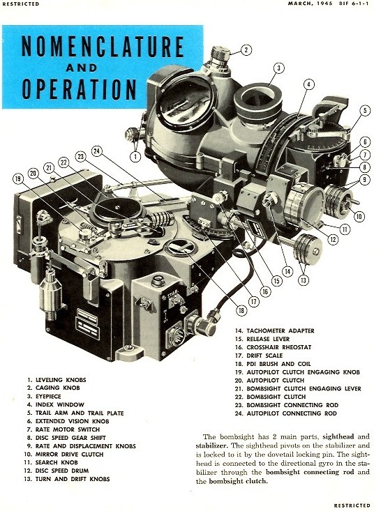
A page from the Bombardier’s Information File (BIF) that describes the components and controls of the Norden bombsight. The Norden bombsight was a highly sophisticated optical/mechanical analog computer used by the United States Army Air Force during World War II, the Korean War, and the Vietnam War to aid the pilot of a bomber aircraft in dropping bombs accurately.

 

的沒落史。這一切可說是『取樣理論』發展的必然結果！『類比』終究會為『數位』所取代。

Sampling (signal processing)

In signal processing, sampling is the reduction of a continuous signal to a discrete signal. A common example is the conversion of a sound wave (a continuous signal) to a sequence of samples (a discrete-time signal).

A sample is a value or set of values at a point in time and/or space.

A sampler is a subsystem or operation that extracts samples from a continuous signal.

A theoretical ideal sampler produces samples equivalent to the instantaneous value of the continuous signal at the desired points.

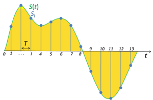
Signal sampling representation. The continuous signal is represented with a green colored line while the discrete samples are indicated by the blue vertical lines.

Theory

Sampling can be done for functions varying in space, time, or any other dimension, and similar results are obtained in two or more dimensions.

For functions that vary with time, let s(t) be a continuous function (or “signal”) to be sampled, and let sampling be performed by measuring the value of the continuous function every T seconds, which is called the sampling interval.^[1]  Then the sampled function is given by the sequence:

s(nT),   for integer values of n.

The sampling frequency or sampling rate, f_s, is the average number of samples obtained in one second (samples per second), thus f_s = 1/T.

Reconstructing a continuous function from samples is done by interpolation algorithms. The Whittaker–Shannon interpolation formula is mathematically equivalent to an ideal lowpass filter whose input is a sequence of Dirac delta functions that are modulated (multiplied) by the sample values. When the time interval between adjacent samples is a constant (T), the sequence of delta functions is called a Dirac comb. Mathematically, the modulated Dirac comb is equivalent to the product of the comb function with s(t). That purely mathematical abstraction is sometimes referred to as impulse sampling.^[2]

Most sampled signals are not simply stored and reconstructed. But the fidelity of a theoretical reconstruction is a customary measure of the effectiveness of sampling. That fidelity is reduced when s(t) contains frequency components whose periodicity is smaller than 2 samples; or equivalently the ratio of cycles to samples exceeds ½ (see Aliasing). The quantity ½ cycles/sample × f_s samples/sec = f_s/2 cycles/sec (hertz) is known as the Nyquist frequency of the sampler. Therefore, s(t) is usually the output of a lowpass filter, functionally known as an anti-aliasing filter. Without an anti-aliasing filter, frequencies higher than the Nyquist frequency will influence the samples in a way that is misinterpreted by the interpolation process.^[3]

───

Whittaker–Shannon interpolation formula

The Whittaker–Shannon interpolation formula or sinc interpolation is a method to construct a continuous-time bandlimited function from a sequence of real numbers. The formula dates back to the works of E. Borel in 1898, and E. T. Whittaker in 1915, and was cited from works of J. M. Whittaker in 1935, and in the formulation of the Nyquist–Shannon sampling theorem by Claude Shannon in 1949. It is also commonly called Shannon’s interpolation formula and Whittaker’s interpolation formula. E. T. Whittaker, who published it in 1915, called it the Cardinal series.

Definition

Given a sequence of real numbers, x[n], the continuous function

(where “sinc” denotes the normalized sinc function) has a Fourier transform, X(f), whose non-zero values are confined to the region |f| ≤ 1/(2T).  When parameter T has units of seconds, the bandlimit, 1/(2T), has units of cycles/sec (hertz). When the x[n] sequence represents time samples, at interval T, of a continuous function, the quantity f_s = 1/T is known as the sample rate, and f_s/2 is the corresponding Nyquist frequency. When the sampled function has a bandlimit, B, less than the Nyquist frequency, x(t) is a perfect reconstruction of the original function. (See Sampling theorem.) Otherwise, the frequency components above the Nyquist frequency “fold” into the sub-Nyquist region of X(f), resulting in distortion. (See Aliasing.)

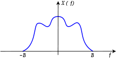
Fourier transform of a bandlimited function.

───

 

事實上『取樣』原理也是深入 Miller Puckette 先生之書，很重要的『概念』之一。因為這『取樣』正是此一『聲音』之『數據流』的源頭。經過 Pd 『箱子』的 處理後，創新且產生『類比』之『音聲 』。