無事不登三寶殿，無因何故寫文章？ Michael Nielsen 先生行文筆法真不可逆料也︰

Softmax

In this chapter we’ll mostly use the cross-entropy cost to address the problem of learning slowdown. However, I want to briefly describe another approach to the problem, based on what are called softmax layers of neurons. We’re not actually going to use softmax layers in the remainder of the chapter, so if you’re in a great hurry, you can skip to the next section. However, softmax is still worth understanding, in part because it’s intrinsically interesting, and in part because we’ll use softmax layers in Chapter 6, in our discussion of deep neural networks.

The idea of softmax is to define a new type of output layer for our neural networks. It begins in the same way as with a sigmoid layer, by forming the weighted inputs* *In describing the softmax we’ll make frequent use of notation introduced in the last chapter. You may wish to revisit that chapter if you need to refresh your memory about the meaning of the notation. $z^L_j = \sum_{k} w^L_{jk} a^{L-1}_k + b^L_j$ $z_{j}^{L} = \sum_{k} w_{j k}^{L} a_{k}^{L - 1} + b_{j}^{L}$ . However, we don’t apply the sigmoid function to get the output. Instead, in a softmax layer we apply the so-called softmax function to the $z^L_j$ $z_{j}^{L}$ . According to this function, the activation $a^L_j$ $a_{j}^{L}$ of the $j$ $j$ th output neuron is

a^L_j = \frac{e^{z^L_j}}{\sum_k e^{z^L_k}}, \ \ \ \ (78)

where in the denominator we sum over all the output neurons.

If you’re not familiar with the softmax function, Equation (78) may look pretty opaque. It’s certainly not obvious why we’d want to use this function. And it’s also not obvious that this will help us address the learning slowdown problem. To better understand Equation (78), suppose we have a network with four output neurons, and four corresponding weighted inputs, which we’ll denote $z^L_1, z^L_2, z^L_3$ $z_{1}^{L}, z_{2}^{L}, z_{3}^{L}$ , and $z^L_4$ $z_{4}^{L}$ . Shown below are adjustable sliders showing possible values for the weighted inputs, and a graph of the corresponding output activations. A good place to start exploration is by using the bottom slider to increase $z^L_4$ $z_{4}^{L}$ :

softmax

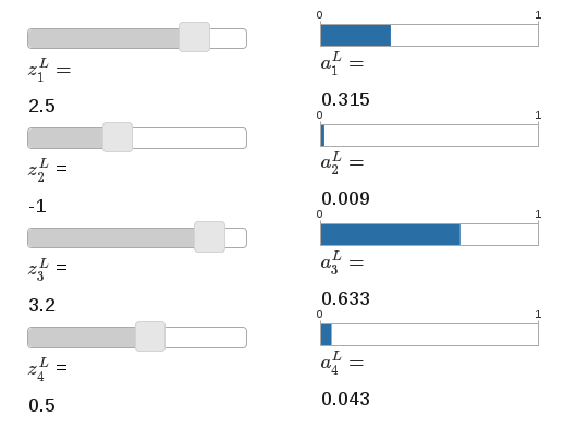
As you increase $z^L_4$ $z_{4}^{L}$ , you’ll see an increase in the corresponding output activation, $a^L_4$ $a_{4}^{L}$ , and a decrease in the other output activations. Similarly, if you decrease $z^L_4$ $z_{4}^{L}$ then $a^L_4$ $a_{4}^{L}$ will decrease, and all the other output activations will increase. In fact, if you look closely, you’ll see that in both cases the total change in the other activations exactly compensates for the change in $a^L_4$ $a_{4}^{L}$ . The reason is that the output activations are guaranteed to always sum up to $1$ $1$ , as we can prove using Equation (78) and a little algebra:

\sum_j a^L_j & = & \frac{\sum_j e^{z^L_j}}{\sum_k e^{z^L_k}} = 1. \ \ \ \ (79)

As a result, if $a^L_4$ $a_{4}^{L}$ increases, then the other output activations must decrease by the same total amount, to ensure the sum over all activations remains $1$ $1$ . And, of course, similar statements hold for all the other activations.

Equation (78) also implies that the output activations are all positive, since the exponential function is positive. Combining this with the observation in the last paragraph, we see that the output from the softmax layer is a set of positive numbers which sum up to $1$ $1$ . In other words, the output from the softmax layer can be thought of as a probability distribution.

The fact that a softmax layer outputs a probability distribution is rather pleasing. In many problems it’s convenient to be able to interpret the output activation $a^L_j$ $a_{j}^{L}$ as the network’s estimate of the probability that the correct output is $j$ $j$ . So, for instance, in the MNIST classification problem, we can interpret $a^L_j$ $a_{j}^{L}$ as the network’s estimated probability that the correct digit classification is $j$ $j$ .

By contrast, if the output layer was a sigmoid layer, then we certainly couldn’t assume that the activations formed a probability distribution. I won’t explicitly prove it, but it should be plausible that the activations from a sigmoid layer won’t in general form a probability distribution. And so with a sigmoid output layer we don’t have such a simple interpretation of the output activations.

若說有說『Softmax』是什麼？僅只有『定義』而已！彷彿沒說？？若說沒說？還有個『動態模擬』可以玩玩！！考之維基百科詞條︰

Softmax function

In mathematics, in particular probability theory and related fields, the softmax function, or normalized exponential,^[1]^:198 is a generalization of the logistic function that “squashes” a $K$ -dimensional vector $\mathbf{z}$ of arbitrary real values to a $K$ -dimensional vector $\sigma(\mathbf{z})$ of real values in the range (0, 1) that add up to 1. The function is given by

\sigma(\mathbf{z})_j = \frac{e^{z_j}}{\sum_{k=1}^K e^{z_k}}

for j = 1, …, K.

The softmax function is the gradient-log-normalizer of the categorical probability distribution. For this reason, the softmax function is used in various probabilistic multiclass classification methods including multinomial logistic regression,^[1]^:206–209 multiclass linear discriminant analysis, naive Bayes classifiers and artificial neural networks.^[2] Specifically, in multinomial logistic regression and linear discriminant analysis, the input to the function is the result of $K$ distinct linear functions, and the predicted probability for the $j$ ‘th class given a sample vector $x$ is:

P(y=j|\mathbf{x}) = \frac{e^{\mathbf{x}^\mathsf{T}\mathbf{w}_j}}{\sum_{k=1}^K e^{\mathbf{x}^\mathsf{T}\mathbf{w}_k}}

This can be seen as the composition of $K$ linear functions $\mathbf{x} \mapsto \mathbf{x}^\mathsf{T}\mathbf{w}_1, \ldots, \mathbf{x} \mapsto \mathbf{x}^\mathsf{T}\mathbf{w}_K$ and the softmax function (where $\mathbf{x}^\mathsf{T}\mathbf{w}$ denotes the inner product of $\mathbf{x}$ and $\mathbf{w}$ ).

Artificial neural networks

In neural network simulations, the softmax function is often implemented at the final layer of a network used for classification. Such networks are then trained under a log loss (or cross-entropy) regime, giving a non-linear variant of multinomial logistic regression.

Since the function maps a vector and a specific index i to a real value, the derivative needs to take the index into account:

\frac{\partial}{\partial q_k}\sigma(\textbf{q}, i) = \dots = \sigma(\textbf{q}, i)(\delta_{ik} - \sigma(\textbf{q}, k))

Here, the Kronecker delta is used for simplicity (cf. the derivative of a sigmoid function, being expressed via the function itself).

See Multinomial logit for a probability model which uses the softmax activation function.

Reinforcement learning

In the field of reinforcement learning, a softmax function can be used to convert values into action probabilities. The function commonly used is:^[3]

P_t(a) = \frac{\exp(q_t(a)/\tau)}{\sum_{i=1}^n\exp(q_t(i)/\tau)} \text{,}

where the action value $q_t(a)$ corresponds to the expected reward of following action a and $\tau$ is called a temperature parameter (in allusion to statistical mechanics). For high temperatures ( $\tau\to \infty$ ), all actions have nearly the same probability and the lower the temperature, the more expected rewards affect the probability. For a low temperature ( $\tau\to 0^+$ ), the probability of the action with the highest expected reward tends to 1.

───

或可得部份習題解答，

Exercise

Construct an example showing explicitly that in a network with a sigmoid output layer, the output activations $a^L_j$ $a_{j}^{L}$ won’t always sum to $1$ $1$ .

We’re starting to build up some feel for the softmax function and the way softmax layers behave. Just to review where we’re at: the exponentials in Equation (78) ensure that all the output activations are positive. And the sum in the denominator of Equation (78) ensures that the softmax outputs sum to $1$ $1$ . So that particular form no longer appears so mysterious: rather, it is a natural way to ensure that the output activations form a probability distribution. You can think of softmax as a way of rescaling the $z^L_j$ $z_{j}^{L}$ , and then squishing them together to form a probability distribution.

Exercises

Monotonicity of softmax Show that $\partial a^L_j / \partial z^L_k$ $\partial a_{j}^{L} / \partial z_{k}^{L}$ is positive if $j = k$ $j = k$ and negative if $j \neq k$ $j \neq k$ . As a consequence, increasing $z^L_j$ $z_{j}^{L}$ is guaranteed to increase the corresponding output activation, $a^L_j$ $a_{j}^{L}$ , and will decrease all the other output activations. We already saw this empirically with the sliders, but this is a rigorous proof.
Non-locality of softmax A nice thing about sigmoid layers is that the output $a^L_j$ $a_{j}^{L}$ is a function of the corresponding weighted input, $a^L_j = \sigma(z^L_j)$ $a_{j}^{L} = σ (z_{j}^{L})$ . Explain why this is not the case for a softmax layer: any particular output activation $a_{j}^{L}$ depends on all the weighted inputs.

Problem

Inverting the softmax layer Suppose we have a neural network with a softmax output layer, and the activations $a^L_j$ $a_{j}^{L}$ are known. Show that the corresponding weighted inputs have the form $z^L_j = \ln a^L_j + C$ $z_{j}^{L} = \ln a_{j}^{L} + C$ , for some constant $C$ $C$ that is independent of $j$ $j$ .

或當知它與『配分函數』淵源匪淺︰

配分函數（英語：Partition function）是一個平衡態統計物理學中經常應用到的概念，經由計算配分函數可以將微觀物理狀態與宏觀物理量相互聯繫起來，而配分函數等價於自由能，與路徑積分在數學上有巧妙的類似。

Partition function (statistical mechanics)

In physics, a partition function describes the statistical properties of a system in thermodynamic equilibrium. Partition functions are functions of the thermodynamic state variables, such as the temperature and volume. Most of the aggregate thermodynamic variables of the system, such as the total energy, free energy, entropy, and pressure, can be expressed in terms of the partition function or its derivatives.

Each partition function is constructed to represent a particular statistical ensemble (which, in turn, corresponds to a particular free energy). The most common statistical ensembles have named partition functions. The canonical partition function applies to a canonical ensemble, in which the system is allowed to exchange heat with the environment at fixed temperature, volume, and number of particles. The grand canonical partition function applies to a grand canonical ensemble, in which the system can exchange both heat and particles with the environment, at fixed temperature, volume, and chemical potential. Other types of partition functions can be defined for different circumstances; see partition function (mathematics) for generalizations. The partition function has many physical meanings, as discussed in Meaning and significance.

Definition

As a beginning assumption, assume that a thermodynamically large system is in thermal contact with the environment, with a temperature T, and both the volume of the system and the number of constituent particles are fixed. This kind of system is called a canonical ensemble. The appropriate mathematical expression for the canonical partition function depends on the degrees of freedom of the system, whether the context is classical mechanics or quantum mechanics, and whether the spectrum of states is discrete or continuous.

Classical discrete system

For a canonical ensemble that is classical and discrete, the canonical partition function is defined as

Z = \sum_{i} \mathrm{e}^{- \beta E_i}

where

i

is the index for the microstates of the system,

\beta

is the thermodynamic beta defined as

\tfrac{1}{k_B T}

E_i

is the total energy of the system in the respective microstate.

Derivation of canonical partition function (classical, discrete)

There are multiple approaches to deriving the partition function. The following derivation follows the powerful and general information-theoretic Jaynesian maximum entropy approach.

According to the second law of thermodynamics, a system assumes a configuration of maximum entropy at thermodynamic equilibrium. We seek a probability distribution of states $\rho_i$ which maximizes the discrete Gibbs entropy

S = - k_B \sum_i \rho_i \ln(\rho_i)

subject to two physical constraints:

1. The probabilities of all states add to unity.

\sum_i \rho_i = 1

2. In the canonical ensemble, the average energy is fixed.

\langle E \rangle = \sum_i \rho_i E_i \equiv U

Using the method of Lagrange multipliers, we write the Lagrangian (or Lagrange function) $\mathcal{L}$ as:

\mathcal{L} = \left( - k_B \sum_i \rho_i \ln(\rho_i) \right) + \lambda_1 \left( \sum_i \rho_i - 1 \right) + \lambda_2 \left( \sum_i \rho_i E_i - U \right)

Differentiating and extremizing $\mathcal{L}$ with respect to $\rho_i$ leads to:

0 = \frac{\partial \mathcal{L}}{\partial \rho_i} = -k_B \ln(\rho_i) - k_B + \lambda_1 + \lambda_2 E_i

Isolating for $\rho_i$ yields:

\rho_i = \exp \left( \frac{-k_B + \lambda_1 + \lambda_2 E_i}{k_B} \right)

To obtain $\lambda_1$ , one substitutes the probability into the first constraint:

\text{[math]}

where $Z$ is defined as the canonical ensemble partition function:

\text{[math]}

Rewriting $\text{[math]}$ in terms of $\text{[math]}$ gives:

\text{[math]}

Rewriting $\text{[math]}$ in terms of $\text{[math]}$ gives:

\text{[math]}

To obtain $\text{[math]}$ , we differentiate $\text{[math]}$ with respect to the average energy $\text{[math]}$ and apply the first law of thermodynamics: