『眼見為憑』，明白統計數據間之局部與全局關係，此乃

安斯庫姆四重奏

安斯庫姆四重奏（Anscombe’s quartet）是四組基本的統計特性一致的數據，但由它們繪製出的圖表則截然不同。每一組數據都包括了11個(x,y)點。這四組數據由統計學家弗朗西斯·安斯庫姆（Francis Anscombe）於1973年構造，他的目的是用來說明在分析數據前先繪製圖表的重要性，以及離群值對統計的影響之大。

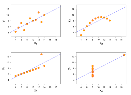
安斯庫姆四重奏的四組數據圖表

這四組數據的共同統計特性如下：

性質	數值
x的平均數	9
x的方差	11
y的平均數	7.50（精確到小數點後兩位）
y的方差	4.122或4.127（精確到小數點後三位）
x與y之間的相關係數	0.816（精確到小數點後三位）
線性回歸線	$\displaystyle y=3.00+0.500x$ （分別精確到小數點後兩位和三位）

在四幅圖中，由第一組數據繪製的圖表（左上圖）是看起來最「正常」的，可以看出兩個隨機變量之間的相關性。從第二組數據的圖表（右上圖）則可以明顯地看出兩個隨機變量間的關係是非線性的。第三組中（左下圖），雖然存在著線性關係，但由於一個離群值的存在，改變了線性回歸線，也使得相關係數從1降至 0.81。最後，在第四個例子中（右下圖），儘管兩個隨機變量間沒有線性關係，但僅僅由於一個離群值的存在就使得相關係數變得很高。

愛德華·塔夫特（Edward Tufte）在他所著的《圖表設計的現代主義革命》（The Visual Display of Quantitative Information）一書的第一頁中，就使用安斯庫姆四重奏來說明繪製數據圖表的重要性。

四組數據的具體取值如下所示。其中前三組數據的x值都相同。

安斯庫姆四重奏
一		二		三		四
x	y	x	y	x	y	x	y
10.0	8.04	10.0	9.14	10.0	7.46	8.0	6.58
8.0	6.95	8.0	8.14	8.0	6.77	8.0	5.76
13.0	7.58	13.0	8.74	13.0	12.74	8.0	7.71
9.0	8.81	9.0	8.77	9.0	7.11	8.0	8.84
11.0	8.33	11.0	9.26	11.0	7.81	8.0	8.47
14.0	9.96	14.0	8.10	14.0	8.84	8.0	7.04
6.0	7.24	6.0	6.13	6.0	6.08	8.0	5.25
4.0	4.26	4.0	3.10	4.0	5.39	19.0	12.50
12.0	10.84	12.0	9.13	12.0	8.15	8.0	5.56
7.0	4.82	7.0	7.26	7.0	6.42	8.0	7.91
5.0	5.68	5.0	4.74	5.0	5.73	8.0	6.89

的主旋律乎？如是者將會知道概念間的關係及其先後次序之重要性吧！

Covariance

In probability theory and statistics, covariance is a measure of the joint variability of two random variables.^[1] If the greater values of one variable mainly correspond with the greater values of the other variable, and the same holds for the lesser values, i.e., the variables tend to show similar behavior, the covariance is positive.^[2] For example, as a balloon is blown up it gets larger in all dimensions. In the opposite case, when the greater values of one variable mainly correspond to the lesser values of the other, i.e., the variables tend to show opposite behavior, the covariance is negative. If a sealed balloon is squashed in one dimension then it will expand in the other two. The sign of the covariance therefore shows the tendency in the linear relationship between the variables. The magnitude of the covariance is not easy to interpret. The normalized version of the covariance, the correlation coefficient, however, shows by its magnitude the strength of the linear relation.

A distinction must be made between (1) the covariance of two random variables, which is a population parameter that can be seen as a property of the joint probability distribution, and (2) the sample covariance, which in addition to serving as a descriptor of the sample, also serves as an estimated value of the population parameter.

Definition

The covariance between two jointly distributed real-valued random variables $X$ and $Y$ with finite second moments is defined as^[3]

\operatorname {cov} (X,Y)=\operatorname {E} {{\big [}(X-\operatorname {E} [X])(Y-\operatorname {E} [Y]){\big ]}},

where $E[X]$ is the expected value of $X$ , also known as the mean of $X$ . The covariance is also sometimes denoted “ $σ$ ”, in analogy to variance. By using the linearity property of expectations, this can be simplified to

{\begin{aligned}\operatorname {cov} (X,Y)&=\operatorname {E} \left[\left(X-\operatorname {E} \left[X\right]\right)\left(Y-\operatorname {E} \left[Y\right]\right)\right]\\&=\operatorname {E} \left[XY-X\operatorname {E} \left[Y\right]-\operatorname {E} \left[X\right]Y+\operatorname {E} \left[X\right]\operatorname {E} \left[Y\right]\right]\\&=\operatorname {E} \left[XY\right]-\operatorname {E} \left[X\right]\operatorname {E} \left[Y\right]-\operatorname {E} \left[X\right]\operatorname {E} \left[Y\right]+\operatorname {E} \left[X\right]\operatorname {E} \left[Y\right]\\&=\operatorname {E} \left[XY\right]-\operatorname {E} \left[X\right]\operatorname {E} \left[Y\right].\end{aligned}}

However, when $\operatorname {E} [XY]\approx \operatorname {E} [X]\operatorname {E} [Y]$ , this last equation is prone to catastrophic cancellation when computed with floating point arithmetic and thus should be avoided in computer programs when the data has not been centered before.^[4] Numerically stable algorithms should be preferred in this case.

Joint probability distribution

In the study of probability, given at least two random variables X, Y, …, that are defined on a probability space, the joint probability distribution for X, Y, … is a probability distribution that gives the probability that each of X, Y, … falls in any particular range or discrete set of values specified for that variable. In the case of only two random variables, this is called a bivariate distribution, but the concept generalizes to any number of random variables, giving a multivariate distribution.

The joint probability distribution can be expressed either in terms of a joint cumulative distribution function or in terms of a joint probability density function (in the case of continuous variables) or joint probability mass function (in the case of discrete variables). These in turn can be used to find two other types of distributions: the marginal distribution giving the probabilities for any one of the variables with no reference to any specific ranges of values for the other variables, and the conditional probability distribution giving the probabilities for any subset of the variables conditional on particular values of the remaining variables.

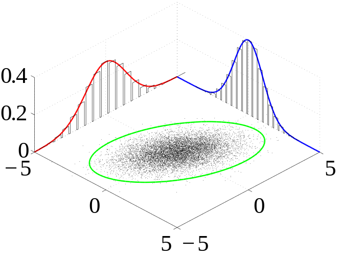
Many sample observations (black) are shown from a joint probability distribution. The marginal densities are shown as well.

Examples

Coin Flips

Consider the flip of two fair coins; let A and B be discrete random variables associated with the outcomes first and second coin flips respectively. If a coin displays “heads” then associated random variable is 1, and is 0 otherwise. The joint probability density function of A and B defines probabilities for each pair of outcomes. All possible outcomes are

(A=0,B=0),(A=0,B=1),(A=1,B=0),(A=1,B=1)

Since each outcome is equally likely the joint probability density function becomes

P(A,B)=1/4

when $A,B\in \{0,1\}$ . Since the coin flips are independent, the joint probability density function is the product of the marginals:

P(A,B)=P(A)P(B)

In general, each coin flip is a Bernoulli trial and the sequence of flips follows a Bernoulli distribution.

Dice Rolls

Consider the roll of a fair die and let A = 1 if the number is even (i.e. 2, 4, or 6) and A = 0 otherwise. Furthermore, let B = 1 if the number is prime (i.e. 2, 3, or 5) and B = 0 otherwise.

	1	2	3	4	5	6
A	0	1	0	1	0	1
B	0	1	1	0	1	0

Then, the joint distribution of A and B, expressed as a probability mass function, is

\mathrm {P} (A=0,B=0)=P\{1\}={\frac {1}{6}},\;\mathrm {P} (A=1,B=0)=P\{4,6\}={\frac {2}{6}},

\mathrm {P} (A=0,B=1)=P\{3,5\}={\frac {2}{6}},\;\mathrm {P} (A=1,B=1)=P\{2\}={\frac {1}{6}}.

These probabilities necessarily sum to 1, since the probability of some combination of A and B occurring is 1.

因此能掌握『統計相關』說何事？

Correlation and dependence

In statistics, dependence or association is any statistical relationship, whether causal or not, between two random variables or two sets of data. Correlation is any of a broad class of statistical relationships involving dependence, though in common usage it most often refers to the extent to which two variables have a linear relationship with each other. Familiar examples of dependent phenomena include the correlation between the physical statures of parents and their offspring, and the correlation between the demand for a product and its price.

Correlations are useful because they can indicate a predictive relationship that can be exploited in practice. For example, an electrical utility may produce less power on a mild day based on the correlation between electricity demand and weather. In this example there is a causal relationship, because extreme weather causes people to use more electricity for heating or cooling; however, correlation is not sufficient to demonstrate the presence of such a causal relationship (i.e., correlation does not imply causation).

Formally, dependence refers to any situation in which random variables do not satisfy a mathematical condition of probabilistic independence. In loose usage, correlation can refer to any departure of two or more random variables from independence, but technically it refers to any of several more specialized types of relationship between mean values. There are several correlation coefficients, often denoted ρ or r, measuring the degree of correlation. The most common of these is the Pearson correlation coefficient, which is sensitive only to a linear relationship between two variables (which may exist even if one is a nonlinear function of the other). Other correlation coefficients have been developed to be more robust than the Pearson correlation – that is, more sensitive to nonlinear relationships.^[1]^[2]^[3] Mutual information can also be applied to measure dependence between two variables.

Pearson’s product-moment coefficient

The most familiar measure of dependence between two quantities is the Pearson product-moment correlation coefficient, or “Pearson’s correlation coefficient”, commonly called simply “the correlation coefficient”. It is obtained by dividing the covariance of the two variables by the product of their standard deviations. Karl Pearson developed the coefficient from a similar but slightly different idea by Francis Galton.^[4]

The population correlation coefficient ρ_X,Y between two random variables X and Y with expected values μ_X and μ_Y and standard deviations σ_X and σ_Y is defined as:

\rho _{X,Y}=\mathrm {corr} (X,Y)={\mathrm {cov} (X,Y) \over \sigma _{X}\sigma _{Y}}={E[(X-\mu _{X})(Y-\mu _{Y})] \over \sigma _{X}\sigma _{Y}},

where E is the expected value operator, cov means covariance, and corr is a widely used alternative notation for the correlation coefficient.

The Pearson correlation is defined only if both of the standard deviations are finite and nonzero. It is a corollary of the Cauchy–Schwarz inequality that the correlation cannot exceed 1 in absolute value. The correlation coefficient is symmetric: corr(X,Y) = corr(Y,X).

The Pearson correlation is +1 in the case of a perfect direct (increasing) linear relationship (correlation), −1 in the case of a perfect decreasing (inverse) linear relationship (anticorrelation),^[5] and some value in the open interval (−1, 1) in all other cases, indicating the degree of linear dependence between the variables. As it approaches zero there is less of a relationship (closer to uncorrelated). The closer the coefficient is to either −1 or 1, the stronger the correlation between the variables.

If the variables are independent, Pearson’s correlation coefficient is 0, but the converse is not true because the correlation coefficient detects only linear dependencies between two variables. For example, suppose the random variable X is symmetrically distributed about zero, and Y = X². Then Y is completely determined by X, so that X and Y are perfectly dependent, but their correlation is zero; they are uncorrelated. However, in the special case when X and Y are jointly normal, uncorrelatedness is equivalent to independence.

If we have a series of n measurements of X and Y written as x_i and y_i for i = 1, 2, …, n, then the sample correlation coefficient can be used to estimate the population Pearson correlation r between X and Y. The sample correlation coefficient is written:

r_{xy}={\frac {\sum \limits _{i=1}^{n}(x_{i}-{\bar {x}})(y_{i}-{\bar {y}})}{(n-1)s_{x}s_{y}}}={\frac {\sum \limits _{i=1}^{n}(x_{i}-{\bar {x}})(y_{i}-{\bar {y}})}{\sqrt {\sum \limits _{i=1}^{n}(x_{i}-{\bar {x}})^{2}\sum \limits _{i=1}^{n}(y_{i}-{\bar {y}})^{2}}}},

where x and y are the sample means of X and Y, and s_x and s_y are the sample standard deviations of X and Y.

This can also be written as:

{\begin{aligned}r_{xy}&={\frac {\sum x_{i}y_{i}-n{\bar {x}}{\bar {y}}}{ns_{x}s_{y}}}\\&={\frac {n\sum x_{i}y_{i}-\sum x_{i}\sum y_{i}}{{\sqrt {n\sum x_{i}^{2}-(\sum x_{i})^{2}}}~{\sqrt {n\sum y_{i}^{2}-(\sum y_{i})^{2}}}}}.\end{aligned}}

If x and y are results of measurements that contain measurement error, the realistic limits on the correlation coefficient are not −1 to +1 but a smaller range.^[6]

For the case of a linear model with a single independent variable, the coefficient of determination (R squared) is the square of r, Pearson’s product-moment coefficient.

通達時間序列『自相關』之計算耶？？

Autocorrelation

Autocorrelation, also known as serial correlation, is the correlation of a signal with a delayed copy of itself as a function of delay. Informally, it is the similarity between observations as a function of the time lag between them. The analysis of autocorrelation is a mathematical tool for finding repeating patterns, such as the presence of a periodic signal obscured by noise, or identifying the missing fundamental frequency in a signal implied by its harmonic frequencies. It is often used in signal processing for analyzing functions or series of values, such as time domain signals.

Unit root processes, trend stationary processes, autoregressive processes, and moving average processes are specific forms of processes with autocorrelation.

Definitions

Different fields of study define autocorrelation differently, and not all of these definitions are equivalent. In some fields, the term is used interchangeably with autocovariance.

Statistics

In statistics, the autocorrelation of a random process is the correlation between values of the process at different times, as a function of the two times or of the time lag. Let X be a stochastic process, and t be any point in time. (t may be an integer for a discrete-time process or a real number for a continuous-time process.) Then X_t is the value (or realization) produced by a given run of the process at time t. Suppose that the process has mean μ_t and variance σ_t² at time t, for each t. Then the definition of the autocorrelation between times s and t is

R(s,t)={\frac {\operatorname {E} [(X_{t}-\mu _{t})(X_{s}-\mu _{s})]}{\sigma _{t}\sigma _{s}}}\,,

where “E” is the expected value operator. Note that this expression is not well-defined for all-time series or processes, because the mean may not exist, or the variance may be zero (for a constant process) or infinite (for processes with distribution lacking well-behaved moments, such as certain types of power law). If the function R is well-defined, its value must lie in the range [−1, 1], with 1 indicating perfect correlation and −1 indicating perfect anti-correlation.

If X_t is a wide-sense stationary process then the mean μ and the variance σ² are time-independent, and further the autocorrelation depends only on the lag between t and s: the correlation depends only on the time-distance between the pair of values but not on their position in time. This further implies that the autocorrelation can be expressed as a function of the time-lag, and that this would be an even function of the lag τ = s − t. This gives the more familiar form

R(\tau )={\frac {\operatorname {E} [(X_{t}-\mu )(X_{t+\tau }-\mu )]}{\sigma ^{2}}},\,

and the fact that this is an even function can be stated as

R(\tau )=R(-\tau ).\,

It is common practice in some disciplines, other than statistics and time series analysis, to drop the normalization by σ² and use the term “autocorrelation” interchangeably with “autocovariance”. However, the normalization is important both because the interpretation of the autocorrelation as a correlation provides a scale-free measure of the strength of statistical dependence, and because the normalization has an effect on the statistical properties of the estimated autocorrelations.

庶幾免於相關、因果間誤謬也！！

Correlation does not imply causation

“Correlation does not imply causation” is a phrase used in statistics to emphasize that a correlation between two variables does not imply that one causes the other.^[1]^[2] Many statistical tests calculate correlation between variables. A few go further, using correlation as a basis for testing a hypothesis of a true causal relationship; examples are the Granger causality test and convergent cross mapping.^{[clarification needed]}

The counter-assumption, that “correlation proves causation,” is considered a questionable cause logical fallacy in that two events occurring together are taken to have a cause-and-effect relationship. This fallacy is also known as cum hoc ergo propter hoc, Latin for “with this, therefore because of this,” and “false cause.” A similar fallacy, that an event that follows another was necessarily a consequence of the first event, is sometimes described as post hoc ergo propter hoc (Latin for “after this, therefore because of this.”).

For example, in a widely studied case, numerous epidemiological studies showed that women taking combined hormone replacement therapy (HRT) also had a lower-than-average incidence of coronary heart disease (CHD), leading doctors to propose that HRT was protective against CHD. But randomized controlled trials showed that HRT caused a small but statistically significant increase in risk of CHD. Re-analysis of the data from the epidemiological studies showed that women undertaking HRT were more likely to be from higher socio-economic groups (ABC1), with better-than-average diet and exercise regimens. The use of HRT and decreased incidence of coronary heart disease were coincident effects of a common cause (i.e. the benefits associated with a higher socioeconomic status), rather than a direct cause and effect, as had been supposed.^[3]

As with any logical fallacy, identifying that the reasoning behind an argument is flawed does not imply that the resulting conclusion is false. In the instance above, if the trials had found that hormone replacement therapy does in fact have a negative incidence on the likelihood of coronary heart disease the assumption of causality would have been correct, although the logic behind the assumption would still have been flawed.

FreeSandal

時間序列︰安斯庫姆四重奏