如果說分明是『假像』！又為什麼能欺騙『視覺』的呢？

【Optical illusion】

An optical illusion (also called a visual illusion) is an illusion caused by the visual system and characterized by visually perceived images that differ from objective reality. The information gathered by the eye is processed in the brain to give a percept that does not tally with a physical measurement of the stimulus source. There are three main types: literal optical illusions that create images that are different from the objects that make them, physiological illusions that are the effects of excessive stimulation of a specific type (brightness, colour, size, position, tilt, movement), and cognitive illusions, the result of unconscious inferences. Pathological visual illusions arise from a pathological exaggeration in physiological visual perception mechanisms causing the aforementioned types of illusions.

Optical illusions are often classified into categories including the physical and the cognitive or perceptual,^[1] and contrasted with optical hallucinations.

Physiological illusions, such as the afterimages^[2] following bright lights, or adapting stimuli of excessively longer alternating patterns (contingent perceptual aftereffect), are presumed to be the effects on the eyes or brain of excessive stimulation or interaction with contextual or competing stimuli of a specific type—brightness, color, position, tile, size, movement, etc. The theory is that a stimulus follows its individual dedicated neural path in the early stages of visual processing, and that intense or repetitive activity in that or interaction with active adjoining channels cause a physiological imbalance that alters perception.

The Hermann grid illusion and Mach bands are two illusions that are best explained using a biological approach. Lateral inhibition, where in the receptive field of the retina light and dark receptors compete with one another to become active, has been used to explain why we see bands of increased brightness at the edge of a color difference when viewing Mach bands. Once a receptor is active, it inhibits adjacent receptors. This inhibition creates contrast, highlighting edges. In the Hermann grid illusion the gray spots appear at the intersection because of the inhibitory response which occurs as a result of the increased dark surround.^[3] Lateral inhibition has also been used to explain the Hermann grid illusion, but this has been disproved.^{[citation needed]} More recent empirical approaches to optical illusions have had some success in explaining optical phenomena with which theories based on lateral inhibition have struggled (e.g. Howe et al. 2005).^[4]

Optical illusion disc which is spun displaying the illusion of motion of a man bowing and a woman curtsying to each other in a circle at the outer edge of the disc, 1833

 

如是所謂『眼見為憑』還須一番思辨的吧？？

之前我們談過『海市蜃樓』現象，在此特別介紹一個也叫做『海市蜃樓』的光學玩具︰

 

這個玩具只用兩個凹面鏡，人們就可在頂部開口處，見到放在底部中央之小物的立體、全彩、週邊三百六十度之『實像』！！此處並不多說明那個有趣的玩具，因為隨著上面的 LINK ，讀者自能知道的哩。反倒是推薦一篇論文︰

 

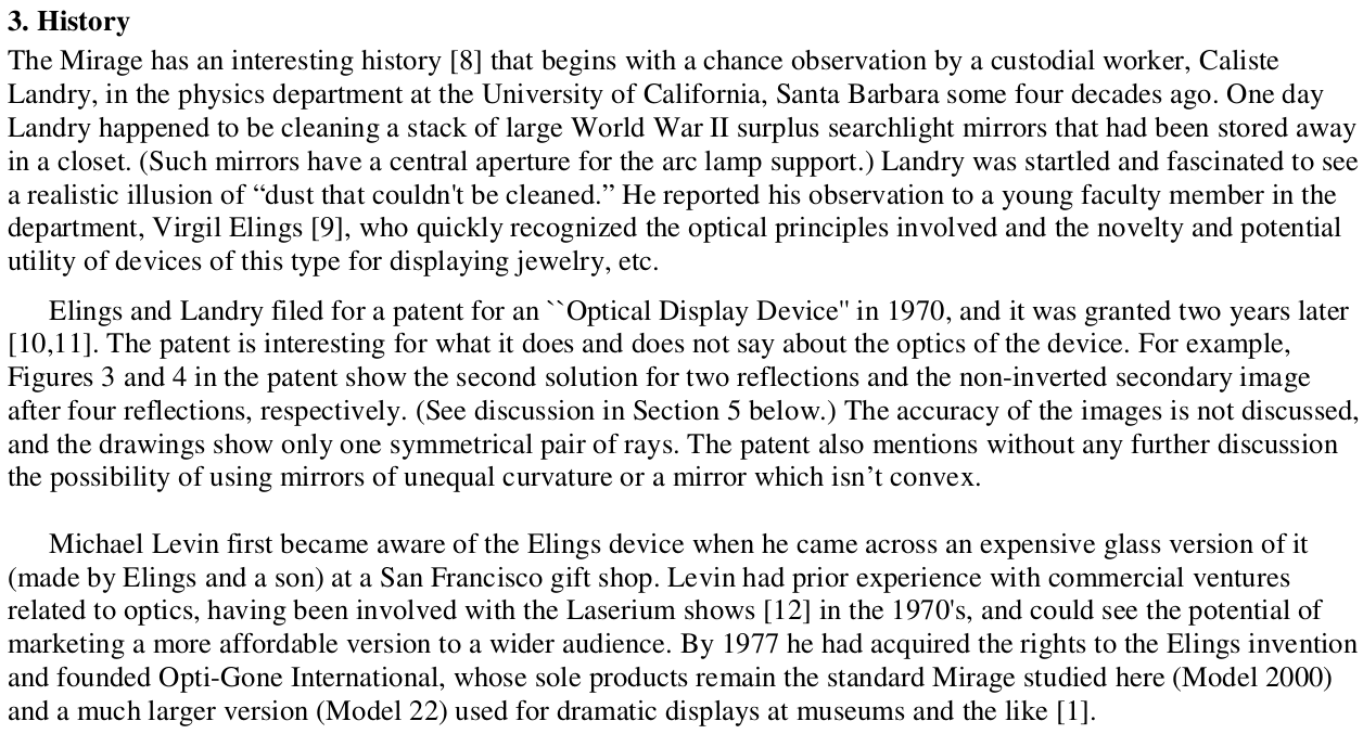
引述文中所言這個現象之神奇發現史︰

 

補註該文裡未言 ABCD 的反射矩陣計算耳。

pi@raspberrypi:~ $ ipython3
Python 3.4.2 (default, Oct 19 2014, 13:31:11) 
Type "copyright", "credits" or "license" for more information.

IPython 2.3.0 -- An enhanced Interactive Python.
?         -> Introduction and overview of IPython's features.
%quickref -> Quick reference.
help      -> Python's own help system.
object?   -> Details about 'object', use 'object??' for extra details.

In [1]: from sympy import *

In [2]: from sympy.physics.optics import FreeSpace, FlatRefraction, ThinLens, GeometricRay, CurvedRefraction, RayTransferMatrix

In [3]: init_printing()

In [4]: d, f, z = symbols('d, f, z')

In [5]: D = RayTransferMatrix(1, d, 0, 1)

In [6]: D
Out[6]: 
⎡1  d⎤
⎢    ⎥
⎣0  1⎦

In [7]: R = RayTransferMatrix(1, 0, -1/f, 1)

In [8]: R
Out[8]: 
⎡ 1   0⎤
⎢      ⎥
⎢-1    ⎥
⎢───  1⎥
⎣ f    ⎦

In [9]: R2 = D*R*D*R*D

In [10]: R2
Out[10]: 
⎡            ⎛  d    ⎞                      ⎛            ⎛  d    ⎞    ⎞    ⎤
⎢          d⋅⎜- ─ + 1⎟ + d                  ⎜          d⋅⎜- ─ + 1⎟ + d⎟    ⎥
⎢  d         ⎝  f    ⎠        ⎛  d    ⎞     ⎜  d         ⎝  f    ⎠    ⎟    ⎥
⎢- ─ + 1 - ───────────────  d⋅⎜- ─ + 1⎟ + d⋅⎜- ─ + 1 - ───────────────⎟ + d⎥
⎢  f              f           ⎝  f    ⎠     ⎝  f              f       ⎠    ⎥
⎢                                                                          ⎥
⎢          d                             ⎛    d        ⎞                   ⎥
⎢        - ─ + 1                         ⎜  - ─ + 1    ⎟                   ⎥
⎢          f       1                     ⎜    f       1⎟   d               ⎥
⎢      - ─────── - ─                   d⋅⎜- ─────── - ─⎟ - ─ + 1           ⎥
⎣           f      f                     ⎝     f      f⎠   f               ⎦

In [11]: R2.B
Out[11]: 
                ⎛            ⎛  d    ⎞    ⎞    
                ⎜          d⋅⎜- ─ + 1⎟ + d⎟    
  ⎛  d    ⎞     ⎜  d         ⎝  f    ⎠    ⎟    
d⋅⎜- ─ + 1⎟ + d⋅⎜- ─ + 1 - ───────────────⎟ + d
  ⎝  f    ⎠     ⎝  f              f       ⎠    

In [12]: solve(R2.B, d)
Out[12]: [0, f, 3⋅f]

In [13]: R4 = D*R*D*R*D*R*D*R*D

In [14]: solve(R4.B, d)
Out[14]: 
⎡     ⎛  √5   3⎞    ⎛  √5   5⎞    ⎛√5   3⎞    ⎛√5   5⎞⎤
⎢0, f⋅⎜- ── + ─⎟, f⋅⎜- ── + ─⎟, f⋅⎜── + ─⎟, f⋅⎜── + ─⎟⎥
⎣     ⎝  2    2⎠    ⎝  2    2⎠    ⎝2    2⎠    ⎝2    2⎠⎦

In [15]: