「懸鉤子」的全部文章

數字派 NumPy ︰陣列運算《一》

何謂陣列運算呢?維基百科詞條這麼說︰

Array programming

In computer science, array programming refers to solutions which allow the application of operations to an entire set of values at once. Such solutions are commonly used in scientific and engineering settings.

Modern programming languages that support array programming (also known as vector or multidimensional languages) have been engineered specifically to generalize operations on scalars to apply transparently to vectors, matrices, and higher-dimensional arrays. These include Fortran 90, Mata, MATLAB, Analytica, TK Solver (as lists), Octave, R, Cilk Plus, Julia, Perl Data Language (PDL), Wolfram Language, and the NumPy extension to Python. In these languages, an operation that operates on entire arrays can be called a vectorized operation,[1] regardless of whether it is executed on a vector processor or not.

Array programming primitives concisely express broad ideas about data manipulation. The level of concision can be dramatic in certain cases: it is not uncommon to find array programming language one-liners that require more than a couple of pages of Java code.[2]

Concepts of array

The fundamental idea behind array programming is that operations apply at once to an entire set of values. This makes it a high-level programming model as it allows the programmer to think and operate on whole aggregates of data, without having to resort to explicit loops of individual scalar operations.

Iverson described the rationale behind array programming (actually referring to APL) as follows:[3]

most programming languages are decidedly inferior to mathematical notation and are little used as tools of thought in ways that would be considered significant by, say, an applied mathematician.

The thesis is that the advantages of executability and universality found in programming languages can be effectively combined, in a single coherent language, with the advantages offered by mathematical notation. it is important to distinguish the difficulty of describing and of learning a piece of notation from the difficulty of mastering its implications. For example, learning the rules for computing a matrix product is easy, but a mastery of its implications (such as its associativity, its distributivity over addition, and its ability to represent linear functions and geometric operations) is a different and much more difficult matter.

Indeed, the very suggestiveness of a notation may make it seem harder to learn because of the many properties it suggests for explorations.

[…] Users of computers and programming languages are often concerned primarily with the efficiency of execution of algorithms, and might, therefore, summarily dismiss many of the algorithms presented here. Such dismissal would be short-sighted since a clear statement of an algorithm can usually be used as a basis from which one may easily derive a more efficient algorithm.

The basis behind array programming and thinking is to find and exploit the properties of data where individual elements are similar or adjacent. Unlike object orientation which implicitly breaks down data to its constituent parts (or scalar quantities), array orientation looks to group data and apply a uniform handling.

Function rank is an important concept to array programming languages in general, by analogy to tensor rank in mathematics: functions that operate on data may be classified by the number of dimensions they act on. Ordinary multiplication, for example, is a scalar ranked function because it operates on zero-dimensional data (individual numbers). The cross product operation is an example of a vector rank function because it operates on vectors, not scalars. Matrix multiplication is an example of a 2-rank function, because it operates on 2-dimensional objects (matrices). Collapse operators reduce the dimensionality of an input data array by one or more dimensions. For example, summing over elements collapses the input array by 1 dimension.


不過讀來彷彿是懂非懂!舉個例講︰如果

y_i = f(x_i) ,假設

\vec{x} = [x_0, x_1, \cdots , x_{n-1}] ,那麼可得

\vec{y} = f(\vec{x}), \ where \ \vec{y} = [y_0, y_1, \cdots , y_{n-1}]

豈不好耶?☆

既簡明又清楚,不必費神多寫程式也!◎

或此正是派生『串列綜合表達式』概念之濫觴乎?!

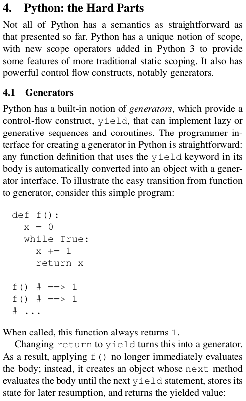
5.1.3. List Comprehensions

List comprehensions provide a concise way to create lists. Common applications are to make new lists where each element is the result of some operations applied to each member of another sequence or iterable, or to create a subsequence of those elements that satisfy a certain condition.

For example, assume we want to create a list of squares, like:

>>> squares = []
>>> for x in range(10):
...     squares.append(x**2)
...
>>> squares
[0, 1, 4, 9, 16, 25, 36, 49, 64, 81]

Note that this creates (or overwrites) a variable named x that still exists after the loop completes. We can calculate the list of squares without any side effects using:

squares = list(map(lambda x: x**2, range(10)))

or, equivalently:

squares = [x**2 for x in range(10)]

which is more concise and readable.

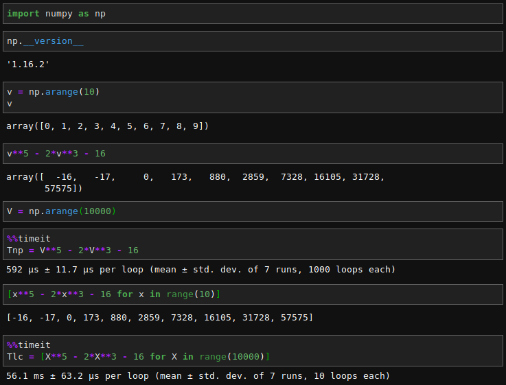
好雖是好,萬一陣列太大,計算『效能』焉能不顧呢☻


數字派 NumPy ︰楔子

最近讀了一本十分受用的書

From Python to Numpy

data/cc.large.png data/by.large.png data/sa.large.png data/nc.large.png

 
Latest version – May 2017
data/cubes.png

There are already a fair number of books about Numpy (see Bibliography) and a legitimate question is to wonder if another book is really necessary. As you may have guessed by reading these lines, my personal answer is yes, mostly because I think there is room for a different approach concentrating on the migration from Python to Numpy through vectorization. There are a lot of techniques that you don’t find in books and such techniques are mostly learned through experience. The goal of this book is to explain some of these techniques and to provide an opportunity for making this experience in the process.

Website: http://www.labri.fr/perso/nrougier/from-python-to-numpy


心想雖然所寫文本也常引用這個派生程式庫『數字派』

NumPy

NumPy (pronounced /ˈnʌmp/ (NUM-py) or sometimes /ˈnʌmpi/[2][3] (NUM-pee)) is a library for the Python programming language, adding support for large, multi-dimensional arrays and matrices, along with a large collection of high-level mathematical functions to operate on these arrays. The ancestor of NumPy, Numeric, was originally created by Jim Hugunin with contributions from several other developers. In 2005, Travis Oliphantcreated NumPy by incorporating features of the competing Numarray into Numeric, with extensive modifications. NumPy is open-source software and has many contributors.

History

The Python programming language was not initially designed for numerical computing, but attracted the attention of the scientific and engineering community early on, so that a special interest group called matrix-sig was founded in 1995 with the aim of defining an array computing package. Among its members was Python designer and maintainer Guido van Rossum, who implemented extensions to Python’s syntax (in particular the indexing syntax) to make array computing easier.[4]

An implementation of a matrix package was completed by Jim Fulton, then generalized by Jim Hugunin to become Numeric,[4] also variously called Numerical Python extensions or NumPy.[5][6] Hugunin, a graduate student at Massachusetts Institute of Technology (MIT),[6]:10 joined the Corporation for National Research Initiatives (CNRI) to work on JPython in 1997[4] leaving Paul Dubois of Lawrence Livermore National Laboratory (LLNL) to take over as maintainer.[6]:10 Other early contributors include David Ascher, Konrad Hinsen and Travis Oliphant.[6]:10

A new package called Numarray was written as a more flexible replacement for Numeric.[7] Like Numeric, it is now deprecated.[8][9] Numarray had faster operations for large arrays, but was slower than Numeric on small ones,[10] so for a time both packages were used for different use cases. The last version of Numeric v24.2 was released on 11 November 2005 and numarray v1.5.2 was released on 24 August 2006.[11]

There was a desire to get Numeric into the Python standard library, but Guido van Rossum decided that the code was not maintainable in its state then.[when?][12]

In early 2005, NumPy developer Travis Oliphant wanted to unify the community around a single array package and ported Numarray’s features to Numeric, releasing the result as NumPy 1.0 in 2006.[7] This new project was part of SciPy. To avoid installing the large SciPy package just to get an array object, this new package was separated and called NumPy. Support for Python 3 was added in 2011 with NumPy version 1.5.0.[13]

In 2011, PyPy started development on an implementation of the NumPy API for PyPy.[14] It is not yet fully compatible with NumPy.[15]


卻是隨手拿來,未曾通盤介紹此一 Python 『數值方法』核心且重要的 package 

Scipy.org

NumPy

 NumPy is the fundamental package for scientific computing with Python. It contains among other things:
  • a powerful N-dimensional array object
  • sophisticated (broadcasting) functions
  • tools for integrating C/C++ and Fortran code
  • useful linear algebra, Fourier transform, and random number capabilities

Besides its obvious scientific uses, NumPy can also be used as an efficient multi-dimensional container of generic data. Arbitrary data-types can be defined. This allows NumPy to seamlessly and speedily integrate with a wide variety of databases.

NumPy is licensed under the BSD license, enabling reuse with few restrictions.


今日逢緣興起,說說『數字派』理念點滴,講講其與『科學派』 SciPy 生態系關係︰

SciPy (pronounced “Sigh Pie”) is a Python-based ecosystem of open-source software for mathematics, science, and engineering. In particular, these are some of the core packages:

  • numpy

    NumPy

    Base N-dimensional array package

  • scipy

    SciPy library

    Fundamental library for scientific computing

  • matplotlib

    Matplotlib

    Comprehensive 2D Plotting

  • ipython

    IPython

    Enhanced Interactive Console

  • sympy

    Sympy

    Symbolic mathematics

  • pandas badge

    pandas

    Data structures & analysis

1. Getting started with Python for science

This part of the Scipy lecture notes is a self-contained introduction to everything that is needed to use Python for science, from the language itself, to numerical computing or plotting.

……

………


願能方便踏腳,特為記。


Rock It 《ML》JupyterLab 【戊】 Julia …

多年來,人們為著不同的目的,創造新的計算機語言。無論自己用或不用,聽聽專家意見總有益處乎?

/julia-mit

Julia for Numerical Computation in MIT Courses

Several MIT courses involving numerical computation, including 18.06, 18.303, 18.330, 18.335/6.337, 18.337/6.338, and18.338, are beginning to use Julia, a fairly new language for technical computing. This page is intended to supplement the Julia documentation with some simple tutorials on installing and using Julia targeted at MIT students. See also our Julia cheatsheet listing a few basic commands, as well as the Learn Julia in Y minutes tutorial page.

In particular, we will be using Julia in the IJulia browser-based enviroment, which leverages your web browser and IPython to provide a rich environment combining code, graphics, formatted text, and even equations, with sophisticated plots via Matplotlib.

See also Viral Shah’s Julia slides and the January 2013 Julia Tutorial videos.

Why Julia?

Traditionally, these sorts of courses at MIT have used Matlab, a high-level environment for numerical computation. Other possibilities might be Scientific Python (the Python language plus numerical libraries), GNU R, and many others. Julia is another high-level free/open-source language for numerical computing in the same spirit, with a rich set of built-in types and libraries for working with linear algebra and other types of computations, with a syntax that is superficially reminiscent of Matlab’s.

High-level dynamic programming languages (as opposed to low-level languages like C or static languages like Java) are essential for interactive exploration of computational science. They allow you to play with matrices, computations on large datasets, plots, and so on without having to worry about managing memory, declaring types, or other minutiae—you can open up a window and start typing commands to immediately get results.

The traditional problem with high-level dynamic languages, however, is that they are slow: as soon as you run into a problem that cannot easily be expressed in terms of built-in library functions operating on large blocks of data (“vectorized” code), you find that your code is suddenly orders of magnitude slower that equivalent code in a low-level language. The typical solution has been to switch to another language (e.g. C or Fortran) to write key computational kernels, calling these from the high-level language (e.g. Matlab or Python) as needed, but this is vastly more difficult than writing code purely in a high-level language and imposes a steep barrier on anyone hoping to transition from casual experimentation to “serious” numerical computation. Julia mostly eliminates this issue, because it is carefully designed to exploit a “just-in-time compiler” called LLVM, making it possible to write high-level code in Julia that achieves near-C speed. (It also means that we can perform meaningful performance experiments easily in courses where this matters, e.g. in 18.335.)

Speed, while avoiding the “two-language” problem of requiring C or Fortran for critical code, is the initial draw of Julia, but there are a few other nice points. Unlike Matlab, it is free/open-source software, which eliminates licensing headaches and allows you to look inside the Julia implementation to see how it works (since Julia is mostly written in Julia, its code is much more readable than a language like Python that is largely implemented in low-level C). For calling existing code, it has easy facilities to call external C or Fortran libraries or to call Python libraries. Multiple dispatch makes it especially easy to overload operations and functions for new types (e.g. to add new vector or numeric types). Julia’s built-in metaprogramming facilities make it easy to write code that generates other code, essentially allowing you to extend the language as needed. And so on…


因此補筆

/IJulia.jl

Julia kernel for Jupyter

IJulia logo

Build Status Build status

IJulia

IJulia is a Julia-language backend combined with the Jupyter interactive environment (also used by IPython). This combination allows you to interact with the Julia language using Jupyter/IPython’s powerful graphical notebook, which combines code, formatted text, math, and multimedia in a single document. It also works with JupyterLab, a Jupyter-based integrated development environment for notebooks and code.

(IJulia notebooks can also be re-used in other Julia code via the NBInclude package.)

Installation

First, download Julia version 0.7 or later and run the installer. Then run the Julia application (double-click on it); a window with ajulia> prompt will appear. At the prompt, type:

using Pkg
Pkg.add("IJulia")

to install IJulia.

This process installs a kernel specification that tells Jupyter (or JupyterLab) etcetera how to launch Julia.

Pkg.add("IJulia") does not actually install Jupyter itself. You can install Jupyter if you want, but it can also be installed automatically when you run IJulia.notebook() below. (You can force it to use a specific jupyter installation by setting ENV["JUPYTER"] to the path of the jupyter program before Pkg.add, or before running Pkg.build("IJulia"); your preference is remembered on subsequent updates.


安裝及驗證︰


順道告知偶見一書

/ThinkJulia.jl

Port of the book Think Python to the Julia programming language

ThinkJulia.jl

Port of the book Think Python to the Julia programming language: online version


或止心頭『餘波蕩漾』徘徊也!


Rock It 《ML》JupyterLab 【戊】 Julia

在結束 Rock It《ML》文本系列前,略為介紹

Julia (programming language)

Julia is a high-level general-purpose[13] dynamic programming language whose designers intend it to address the needs of high-performance numerical analysis and computational science, without the need of separate compilation to be fast.[14][15][16][17] It is also useful for low-level systems programming,[18] as a specification language,[19] with work being done on client[20] and server web use.[21]

Distinctive aspects of Julia’s design include a type system with parametric polymorphism and types in a fully dynamic programming language and multiple dispatch as its core programming paradigm. It allows concurrent,parallel and distributed computing, and direct calling of C and Fortran libraries without glue code.

Julia is garbage-collected,[22] uses eager evaluation, and includes efficient libraries for floating-point calculations, linear algebra, random number generation, and regular expression matching. Many libraries are available, including some (e.g., for fast Fourier transforms) that were previously bundled with Julia and are now separate.[23]

History

Work on Julia was started in 2009, by Jeff Bezanson, Stefan Karpinski, Viral B. Shah, and Alan Edelman, who set out to create a free language that was both high-level and fast. On 14 February 2012 the team launched a website with a blog post explaining the language’s mission.[24] In an interview with Infoworld in April 2012, Karpinski said of the name “Julia”: “There’s no good reason, really. It just seemed like a pretty name.”[25] Bezanson said he chose the name on the recommendation of a friend.[26]

Since the 2012 launch, the Julia community has grown, with over 3,200,000 downloads as of January 2019[27]. The Official Julia Docker images have seen over 1,000,000 downloads.[28]. The JuliaCon[29] academic conference for Julia users and developers has been held annually since 2014.

Version 0.3 was released in August 2014, version 0.4 in October 2015, and version 0.5 in October 2016.[30] Versions 0.5 and earlier are no longer maintained.[31] Julia 0.6 was released in June 2017,[32] and was the stable release version until 8 August 2018.

Both Julia 0.7 (a useful release for testing packages, and knowing how to upgrade them for 1.0[33]) and version 1.0 were released on 8 August 2018. Work on Julia 0.7 was a “huge undertaking” (e.g., because of “entirely new optimizer”), and some changes were made to the syntax (with the syntax now stable, and same for 1.x and 0.7) and semantics; the iteration interface was simplified.[34]

The release candidate for Julia 1.0 (Julia 1.0.0-rc1) was released on 7 August 2018, and the final version a day later. The team has stated code that runs without warnings on Julia 0.7 will run identically on Julia 1.0.[35]

Julia 1.1 was released on 21 January 2019 with, e.g., a new “exception stack” language feature. As promised (by the semantic versioning Julia, and many of the external packages, follows) all old syntax from Julia 1.0 should still work, while Julia 1.1 may not work in Julia 1.0. There are mostly non-breaking additions to the standard library, while there are some small changes explained in Julia’s NEWS file.

Bugfix releases are expected roughly monthly, for Julia 1.1.x and 1.0.x (1.0.x currently has long-term support; for at least a year) and Julia 1.0.1, 1.0.2, and 1.0.3 have followed that schedule (no such bugfix releases in the pipeline for 0.7-release). Julia 1.2 is due 15 March 2019.[36]


以求完整也。

有興趣讀者可造訪其網頁,讀讀

Julia in a Nutshell

Julia is fast!

Julia was designed from the beginning for high performance. Julia programs compile to efficient native code for multiple platforms via LLVM.

Dynamic

Julia is dynamically-typed, feels like a scripting language, and has good support for interactive use.

Optionally typed

Julia has a rich language of descriptive datatypes, and type declarations can be used to clarify and solidify programs.

General

Julia uses multiple dispatch as a paradigm, making it easy to express many object-oriented and functional programming patterns. The standard library provides asynchronous I/O, process control, logging, profiling, a package manager, and more.

Easy to use

Julia has high level syntax, making it an accessible language for programmers from any background or experience level.


有個初步了解。

ROCK 64 上

Download Julia

Long-term support release (v1.0.3)

Users updating code written on older versions to work with 1.0 may be interested in using Julia 0.7 during the upgrade process, available on the old releases page. It is a transitional release that provides deprecation warnings for functionality that differs between Julia 0.6 and 1.0.


安裝辦法如下︰

wget https://julialang-s3.julialang.org/bin/linux/aarch64/1.0/julia-1.0.3-linux-aarch64.tar.gz

tar -zxvf julia-1.0.3-linux-aarch64.tar.gz

ln -s /home/rock64/julia-1.0.3/bin/julia /usr/bin/julia


然後動手吧☆

Getting Started

Julia installation is straightforward, whether using precompiled binaries or compiling from source. Download and install Julia by following the instructions at https://julialang.org/downloads/.

The easiest way to learn and experiment with Julia is by starting an interactive session (also known as a read-eval-print loop or “REPL”) by double-clicking the Julia executable or running julia from the command line:

rock64@rock64:~$ julia 
               _
   _       _ _(_)_     |  Documentation: https://docs.julialang.org
  (_)     | (_) (_)    |
   _ _   _| |_  __ _   |  Type "?" for help, "]?" for Pkg help.
  | | | | | | |/ _` |  |
  | | |_| | | | (_| |  |  Version 1.0.3 (2018-12-18)
 _/ |\__'_|_|_|\__'_|  |  Official https://julialang.org/ release
|__/                   |

julia> 1 + 2
3

julia> ans
3

julia>

To exit the interactive session, type CTRL-D (press the Control/^ key together with the d key), or type exit(). When run in interactive mode, julia displays a banner and prompts the user for input. Once the user has entered a complete expression, such as 1 + 2, and hits enter, the interactive session evaluates the expression and shows its value. If an expression is entered into an interactive session with a trailing semicolon, its value is not shown. The variable ans is bound to the value of the last evaluated expression whether it is shown or not. The ans variable is only bound in interactive sessions, not when Julia code is run in other ways.


Rock It 《ML》JupyterLab 【丁】Code《七》語義【六】解讀‧五

想要了解派生『裝飾子』者,單靠文法定義是不足的︰

The current syntax for function decorators as implemented in Python 2.4a2 is:

@dec2
@dec1
def func(arg1, arg2, ...):
    pass

This is equivalent to:

def func(arg1, arg2, ...):
    pass
func = dec2(dec1(func))

without the intermediate assignment to the variable func. The decorators are near the function declaration. The @ sign makes it clear that something new is going on here.

首要清楚知道『函數』是什麼?

比方說《潜入派生》 Dive into Python 第二章第四節

《 2.4. Everything Is an Object 》講︰

2.4.2. What’s an Object?

Everything in Python is an object, and almost everything has attributes and methods. All functions have a built-in attribute __doc__, which returns the doc string defined in the function’s source code. The sys module is an object which has (among other things) an attribute called path. And so forth.

Still, this begs the question. What is an object? Different programming languages define “object” in different ways. In some, it means that all objects must have attributes and methods; in others, it means that all objects are subclassable. In Python, the definition is looser; some objects have neither attributes nor methods (more on this in Chapter 3), and not all objects are subclassable (more on this in Chapter 5). But everything is an object in the sense that it can be assigned to a variable or passed as an argument to a function (more in this in Chapter 4).

This is so important that I’m going to repeat it in case you missed it the first few times: everything in Python is an object. Strings are objects. Lists are objects. Functions are objects. Even modules are objects.

那麼我們將如何理解『在派生中,一切皆是物件。』這句話呢?要是不深入『派生』的『語法』以及『語意』,只依靠著『語用』根本是不足以『回答』的吧!而且不同的『程式語言』,『口號』不同,『哲學』也不一樣!!Python 號稱『多典範』,『程序』為主的寫作、『物件』中心之編程,『泛函式』概念的淺嚐,……等等,也許可以這麼說︰

『派生』支持的『作法』,讓它『語法』上『方便容易』。

『派生』不支持的『行事』,也可『己選自擇』的『表現』。

─── 《【鼎革‧革鼎】︰ RASPBIAN STRETCH 《六之 J.2A 》


千里來龍,此處結穴!

我們已經看到

 MarioLANG 符號結構之語法可離意欲表達的語義十分遙遠。

或將斟酌使用不同語言翻譯解構情事?

人們將如何『預約』未來,又怎麼『翻譯』過去呢?

Li Bai

A Quiet Night Thought

In front of my bed, there is bright moonlight.
It appears to be frost on the ground.
I lift my head and gaze at the August Moon,
I lower my head and think of my hometown.


Contemplation

Moon twilight approaches, coating the ground through the window,
Resembles a touch of frost,
Moon at the window,
Taking me back to where I am from.

李白

静夜思

床前明月光
疑是地上霜
舉頭望明月
低頭思故鄉

假使將李白的《靜夜思》翻譯成英文,藉由『中英對照』,是否更能『理解』原作之『意境』呢?還是會少了點『』的『味道』??或許這個『利弊得失』就落在︰

『文化』之『盲點』,常顯現在『意義』的『忽略』之中。

『人文』之『偏見』,普遍藏於『字詞』之『情感』之內。

故而同一『內容』的多種『語言文本』,也許可見那『通常之所不見』


或許萬象『錯綜複雜』,難得『意義確解』哩!

─ 摘自《GOPIGO 小汽車︰格點圖像算術《投影幾何》【五‧線性代數】《導引七‧變換組合 VI‧IV 》


因此能了 {\lambda}_{\pi} lambda-py 所說之困難也︰


不必強求『自我再現』的乎☆

一九三九年美國的道德哲學家 William K. Frankena 於英國分析哲學雜誌《心靈》上批評 George Edward Moore 的『自然主義誤謬』── 』不能用『自然性質』定義 ──,太過『狹隘』,甚至引發了一些人使用『非同義詞』non-synonymous 去定義『』。福蘭肯納認為自然主義者之謬誤根本是『用詞不當』misnomer 的『錯誤』︰他們刻意的將『』定義為所有『自然』的特質,而且『拒絕』把任何『不自然』的東西定義為『── 其實是一種『定義家誤謬』 definist fallacy 。

現今所謂的『定義家謬誤』有三種︰

其一、一定要將『此種』特質定義為『彼類』語詞

如前所言。

其二、堅持使用具有『說服性』的定義

語詞有所謂的『字典定義』,這是語詞的一般意義來源以及語詞的正確用法。時間的變遷與知識之進展,都可能發現『語詞』定義『恰不恰當』或者『是非對錯』的問題。然而『語詞的使用』常常又有『一時』或『一群人』的『約定意義』,就語言的『溝通目的』而言無可厚非。假使有人『議論』時,堅持『某字』或『某詞』一定要回歸『某本字典』或『某人所說』的『意思』大概這樣的議論結果是『沒意思』的吧!

其三、詞語使用前請先定義

有人將這種誤謬稱之為『蘇格拉底誤謬』,在柏拉圖寫的『對話錄』中,蘇格拉底總要求『對話者』對『語詞』下『定義』,試圖『釐清』一般語詞的『含混』詞意或者『歧義』用法,也許這不該算是此類的吧!這裡是講有人在『詞意清晰』的語境裡,依然堅持非要求個『明白的定義』不可,或許最終只能先要他把『『定義』之『定義』先給個清楚的『定義』』了吧!!

如此看來『堅持之堅持』與『定義之定義』,如此種種『□○之□○』是思想上的『僵固點』,人果真是『擇善固執』的嗎??

之前在《測不準原理》一文中,我們談過了揚‧武卡謝維奇的『逆波蘭表示法』,於此我們就利用這種表示法的運算並不需要使用括號的特性,寫一個  Thue 的『非、且、或、則』之邏輯符號的真假表達式之求值演算法︰

P 非  ︰P 的否定,
P Q 且︰PQ 的連言,
P Q 或︰PQ 的選言,
P Q 則︰若 PQ 的斷言。

在程式中『 』是使用者輸入的真假表達式,『』用以顯示單步逆波蘭表示法之堆疊推導進行點,『』表示逆波蘭表示法推導結束處,『』告知使用者推導結束。此時如果只剩下『』或『』表示推導正確完成,否則就是說表達式有錯誤。

───  程式起始 ───

真》非::=假》
假》非::=真》
真真》且::=真》
假真》且::=假》
真假》且::=假》
假假》且::=假》
真真》或::=真》
假真》或::=真》
真假》或::=真》
假假》或::=假》
真真》則::=真》
假真》則::=真》
真假》則::=假》
假假》則::=真》
》真::=真》
》假::=假》
》。::=~!
□::=:::
::=
》□。

─── 程式結束 ───

測試輸入︰

□ = 真非真且假非假或則;真
□ = 真真假假則則非則;假
□ = 假假真真則則且非;真
□ = 假假真真且非;假假假

─── 讀別人寫作的程式,動手寫自己的程式,

嘗試發現裡面之錯誤,理解其中關鍵之要點,

恰是自我再現的程式之路 ───

─── 摘自《自我再現 ── THUE 改寫系統之補充《三》