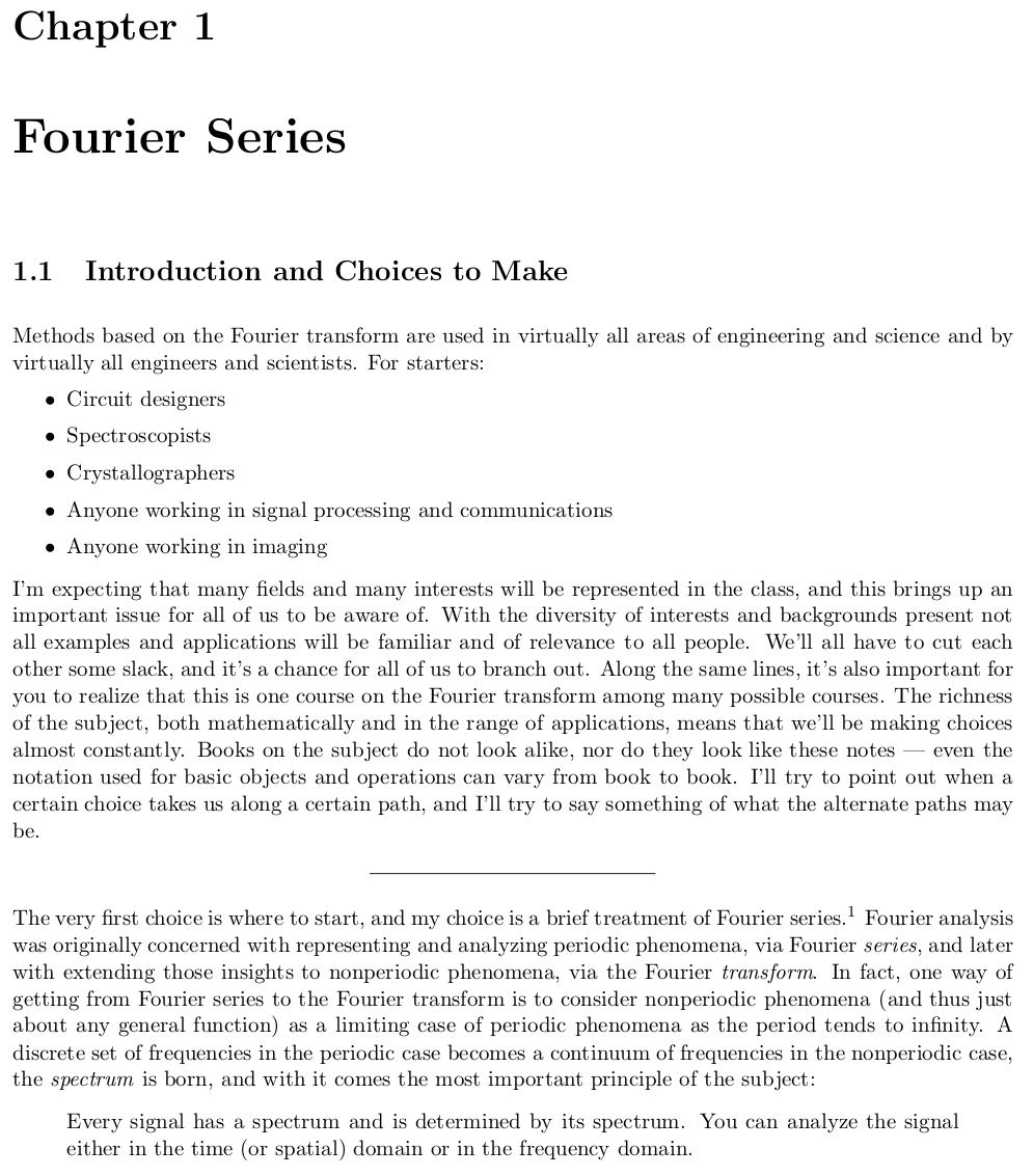
擊鼓，鼓身靜而鼓面動；操琴，琴弦振然琴柱止。這帶出了『物理現象』之

邊值問題

在微分方程中，邊值問題是一個微分方程和一組稱之為邊界條件的約束條件。邊值問題的解通常是符合約束條件的微分方程的解。

物理學中經常遇到邊值問題，例如波動方程等。許多重要的邊值問題屬於Sturm-Liouville問題。這類問題的分析會和微分算子的本徵函數有關。

在實際應用中，邊值問題應當是適定的（即：存在解，解唯一且解會隨著初始值連續的變化）。許多偏微分方程領域的理論提出是為要證明科學及工程應用的許多邊值問題都是適定問題。

最早研究的邊值問題是狄利克雷問題，是要找出調和函數，也就是拉普拉斯方程的解，後來是用狄利克雷原理找到相關的解。

圖中的區域為微分方程有效的區域，且函數在邊界上的值已知

───

數理之探究關聯上『本徵函數』

Eigenfunction

In mathematics, an eigenfunction of a linear operator D defined on some function space is any non-zero function f in that space that, when acted upon by D, is only multiplied by some scaling factor called an eigenvalue. As an equation, this condition can be written as

Df = \lambda f

for some scalar eigenvalue λ.^[1]^[2]^[3] The solutions to this equation may also be subject to boundary conditions that limit the allowable eigenvalues and eigenfunctions.

An eigenfunction is a type of eigenvector.

……

Applications

Vibrating strings

Let $h (x, t)$ denote the sideways displacement of a stressed elastic chord, such as the vibrating strings of a string instrument, as a function of the position $x$ along the string and of time $t$ . Applying the laws of mechanics to infinitesimal portions of the string, the function $h$ satisfies the partial differential equation

\frac{\partial^2 h}{\partial t^2} = c^2\frac{\partial^2 h}{\partial x^2},

which is called the (one-dimensional) wave equation. Here $c$ is a constant speed that depends on the tension and mass of the string.

This problem is amenable to the method of separation of variables. If we assume that $h (x, t)$ can be written as the product of the form $X (x) T (t)$ , we can form a pair of ordinary differential equations:

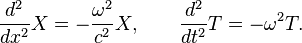
\frac{d^2}{dx^2}X=-\frac{\omega^2}{c^2}X, \qquad \frac{d^2}{dt^2}T=-\omega^2 T.

Each of these is an eigenvalue equation with eigenvalues $-\tfrac{\omega^2}{c^2}$ and $- ω 2$ , respectively. For any values of $ω$ and $c$ , the equations are satisfied by the functions

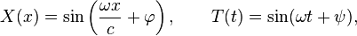
X(x) = \sin\left(\frac{\omega x}{c} + \varphi\right), \qquad T(t) = \sin(\omega t + \psi),

where the phase angles $φ$ and $ψ$ are arbitrary real constants.

If we impose boundary conditions, for example that the ends of the string are fixed at $x = 0$ and $x = L$ , namely $X (0) = X (L) = 0$ , and that $T (0) = 0$ , we constrain the eigenvalues. For these boundary conditions, $sin(φ) = 0$ and $sin(ψ) = 0$ , so the phase angles $φ = ψ = 0$ , and

\sin\left(\frac{\omega L}{c}\right) = 0.

This last boundary condition constrains $ω$ to take a value $ω n = ncπ / L$ , where $n$ is any integer. Thus, the clamped string supports a family of standing waves of the form

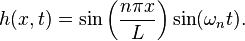
h(x,t) = \sin\left(\frac{n\pi x}{L} \right) \sin(\omega_n t).

In the example of a string instrument, the frequency $ω n$ is the frequency of the $n$ ^th harmonic, which is called the $(n - 1)$ ^th overtone.

Standing_wave

The shape of a standing wave in a string fixed at its boundaries is an example of an eigenfunction of a differential operator. The admissible eigenvalues are governed by the length of the string and determine the frequency of oscillation.

───

終於譜出了『傅立葉分析』之美麗花朵︰

駐波形成

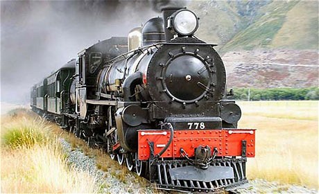
在一輛長列『左行』的火車上有一個很長的『水槽』，上有一向右的『行進波』
$u(x, t) = A(x,\ t)\sin (kx - \omega t + \phi)$
，假使向左的火車與向右之水波速度相同，那麼一位站在月台的『觀察者』將如何描述那個『行進波』的呢？

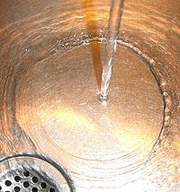
如果觀察水由水龍頭注入水槽的現象，由於水在到達槽底前的流速『較快』，然而到達槽底後水的流速突然的『變慢』，因此會發生『水躍』Hydraulic jump 的現象，此時水之部份動能將轉換為位能，故而在槽底的液面形成『駐波』。這個現象在『河水』的『流速』突然『由快變慢』時也可能發生，因而有人能在『河裡衝浪』，他正站在『駐波』之上！！

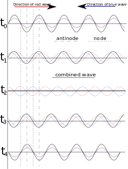
那什麼是『駐波』的呢？比方說一個『不動的』stationary 介質中，向左的波 $u_l(k x + \omega t)$ 與向右的波 $u_r(k x - \omega t)$ 疊加後的『合成波』 $u_l +u_r$ ，在『特定』的『邊界條件』下，被『侷限』在一定『空間區域』內無法前進，因此稱為『駐波』。由於駐波不能傳播能量，它的能量將『儲存』在那個空間區域裡。駐波所在區域，『振幅為零』的點稱為『節點』或『波節』Node ，『振幅最大』的點位於兩『節點』之間，通常叫做『腹點』或『波腹』Antinode。

一根長度 $L$ 震盪的弦上，一個向右的簡諧波 $u_r = u_0 \sin(kx - \omega t)$ ，由於弦的兩頭固定，那個波在右端點也只能『反射』回來，形成了 $u_l = u_0 \sin(kx + \omega t)$ ，此時合成波 $u = u_l + u_r$ 是
$u\; = u_0\sin(kx - \omega t) + u_0 \sin(kx + \omega t)$
，可用三角恆等式簡化為
$u = 2 u_0\cos(\omega t)\sin(kx)$
。此時『時間項』與『空間項』分離，形成『駐波』。在 $kx = n \pi$ 時， $\sin(kx) = 0$ ，此處 $n$ 是整數，這就是『節點』；當 $kx = n \pi + \frac{\pi}{2}$ 時 $\parallel \sin(kx) = 1 \parallel$ ，也就是『腹點』。當然波長 $\lambda$ 就得滿足 $\lambda = \frac {L}{n \pi}$ 的邊界條件。

─── 琴弦擇音而振，苟非知音焉得共鳴。───

───

當更能了解那些滿足 $\lambda = \frac {L}{n \pi}$ 『波長』關係的『頻率』構成了那根『弦』的『泛音』。不同『音色』的『弦』正因此『泛音』頻譜不同而出色。或也將知這也是『正交函數族』 Orthogonal functions 的發展以及『傅立葉級數』之歷史濫觴乎︰

Hilbert space interpretation

In the language of Hilbert spaces, the set of functions { $e_n=e^{inx}$ ; n ∈ Z} is an orthonormal basis for the space L²([− $π$ , $π$ ]) of square-integrable functions of [− $π$ , $π$ ]. This space is actually a Hilbert space with an inner product given for any two elements f and g by

\langle f,\, g \rangle \;\stackrel{\mathrm{def}}{=} \; \frac{1}{2\pi}\int_{-\pi}^{\pi} f(x)\overline{g(x)}\,dx.

The basic Fourier series result for Hilbert spaces can be written as

f=\sum_{n=-\infty}^\infty \langle f,e_n \rangle \, e_n.

This corresponds exactly to the complex exponential formulation given above. The version with sines and cosines is also justified with the Hilbert space interpretation. Indeed, the sines and cosines form an orthogonal set:

400px-Fourier_series_integral_identities

Sines and cosines form an orthonormal set, as illustrated above. The integral of sine, cosine and their product is zero (green and red areas are equal, and cancel out) when m, n or the functions are different, and pi only if m and n are equal, and the function used is the same.

\int_{-\pi}^{\pi} \cos(mx)\, \cos(nx)\, dx = \pi \delta_{mn}, \quad m, n \ge 1, \,

\int_{-\pi}^{\pi} \sin(mx)\, \sin(nx)\, dx = \pi \delta_{mn}, \quad m, n \ge 1

(where δ_mn is the Kronecker delta), and

\int_{-\pi}^{\pi} \cos(mx)\, \sin(nx)\, dx = 0;\,

furthermore, the sines and cosines are orthogonal to the constant function 1. An orthonormal basis for L²([− $π$ , $π$ ]) consisting of real functions is formed by the functions 1 and √2 cos(nx), √2 sin(nx) with n = 1, 2,… The density of their span is a consequence of the Stone–Weierstrass theorem, but follows also from the properties of classical kernels like the Fejér kernel.

───

若非如此，樂器將如何和鳴共奏呢？或終可聞箱子天籟之聲的耶？？！！

若問什麼是『頻譜洩漏』

Spectral leakage

The Fourier transform of a function of time, s(t), is a complex-valued function of frequency, S(f), often referred to as a frequency spectrum. Any linear time-invariant operation on s(t) produces a new spectrum of the form H(f)•S(f), which changes the relative magnitudes and/or angles (phase) of the non-zero values of S(f). Any other type of operation creates new frequency components that may be referred to as spectral leakage in the broadest sense. Sampling, for instance, produces leakage, which we call aliases of the original spectral component. For Fourier transform purposes, sampling is modeled as a product between s(t) and a Dirac comb function. The spectrum of a product is the convolution between S(f) and another function, which inevitably creates the new frequency components. But the term ‘leakage’ usually refers to the effect of windowing, which is the product of s(t) with a different kind of function, the window function. Window functions happen to have finite duration, but that is not necessary to create leakage. Multiplication by a time-variant function is sufficient.

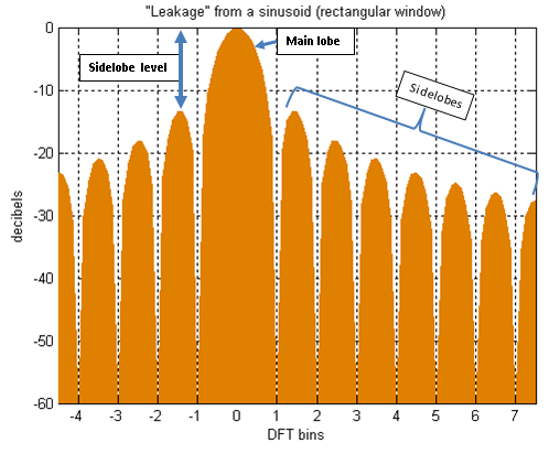
Spectral_leakage_from_a_sinusoid_and_rectangular_window

Zoomed view of spectral leakage.

───

？為什麼會有『洩漏』的呢？？奈何讀來宛如天書耶！！或許因為已不記得了史丹佛大學 Brad Osgood 教授開宗明義講︰傅立葉級數假設『週期現象』！！？？

Fourier-1

Fourier-2

───

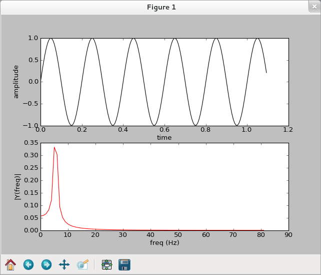
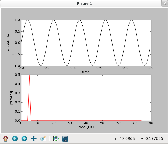
事實上『取樣數據』 $x_1, x_2, x_3, \cdots , x_k , \cdots x_n$ 之 DFT 只是一種『近似描述』，如果再加上不能滿足『頭尾相銜』、『無縫接續』，有不連續性於其間，必有『效應』的乎？？！！

【看圖說故事】

>>> import numpy as np
>>> import matplotlib.pyplot as plt
>>> Fs = 150 #取樣頻率
>>> Ts = 1.0/Fs #取樣間隔
>>> t = np.arange(0,1,Ts) #取樣範圍
>>> ff = 5 #訊號頻率
>>> y = np.sin(2 * np.pi * ff * t) #正弦波
>>> plt.subplot(2,1,1)
<matplotlib.axes.AxesSubplot object at 0x2722d90>
>>> plt.plot(t,y,'k-')
[<matplotlib.lines.Line2D object at 0x2387a90>]
>>> plt.xlabel('time')
<matplotlib.text.Text object at 0x2734c50>
>>> plt.ylabel('amplitude')
<matplotlib.text.Text object at 0x2739bd0>
>>> plt.subplot(2,1,2)
<matplotlib.axes.AxesSubplot object at 0x2755a50>
>>> n = len(y)
>>> k = np.arange(n)
>>> T = n/Fs
>>> frq = k/T
>>> freq = frq[range(n/2)]  #單邊頻域
>>> Y = np.fft.fft(y)/n #FFT 且作歸一化
>>> Y = Y[range(n/2)]
>>> plt.plot(freq, abs(Y), 'r-')
[<matplotlib.lines.Line2D object at 0x2755e10>]
>>> plt.xlabel('freq (Hz)')
<matplotlib.text.Text object at 0x2759cd0>
>>> plt.ylabel('|Y(freq)|')
<matplotlib.text.Text object at 0x275cc50>
>>> plt.show()

Figure sin_p

>>> t = np.arange(0,1.1,Ts)
>>> ff = 5
>>> y = np.sin(2 * np.pi * ff * t)
>>> plt.subplot(2,1,1)
<matplotlib.axes.AxesSubplot object at 0x2afcb90>
>>> plt.plot(t,y,'k-')
[<matplotlib.lines.Line2D object at 0x2d67d50>]
>>> plt.xlabel('time')
<matplotlib.text.Text object at 0x2afa290>
>>> plt.ylabel('amplitude')
<matplotlib.text.Text object at 0x2b136d0>
>>> plt.subplot(2,1,2)
<matplotlib.axes.AxesSubplot object at 0x3033950>
>>> n = len(y)
>>> k = np.arange(n)
>>> T = n/Fs
>>> frq = k/T
>>> freq = frq[range(n/2)]
>>> Y = np.fft.fft(y)/n
>>> Y = Y[range(n/2)]
>>> plt.plot(freq, abs(Y), 'r-')
[<matplotlib.lines.Line2D object at 0x3033d10>]
>>> plt.xlabel('freq (Hz)')
<matplotlib.text.Text object at 0x2af9bd0>
>>> plt.ylabel('|Y(freq)|')
<matplotlib.text.Text object at 0x2af3b50>
>>> plt.show()
>>>

Figure sin_l

日	一	二	三	四	五	六
« 4 月				6 月 »
1	2	3	4	5	6	7
8	9	10	11	12	13	14
15	16	17	18	19	20	21
22	23	24	25	26	27	28
29	30	31

FreeSandal

每日彙整: 2016-05-08

W!o+ 的《小伶鼬工坊演義》︰神經網絡【FFT】四