《花非花》白居易
花非花,霧非霧,
夜半來,天明去,
來如春夢無多時,
去似朝雲無覓處。
香山居士這首詩別出心裁,令人想入非非。莫非
美人花,花非花,似花花解語。
彩雲霧,霧非霧,比霧霧生霞。
春夢恐醒,韶光將逝,如電亦如霧。
朝雲易散,彩霞難留,來去無覓處。
。引人『![]() 』悟吾心乎??感嘆人生幾何耶!!
』悟吾心乎??感嘆人生幾何耶!!
幾人曾賞霧中花?
飄香方知花是花!
春夢朝雲花中霧!
何時才曉霧是霧?
暑中偶偶風雨突至,雷電交加,正是讚嘆自然現象之際,恰合說此萬花尺之時︰
萬花筒非筒?萬花尺非尺!
那位乘天光!千度百回!!
這位伴銀河!百媚千嬌!!
莫要問︰乾坤尺筒何時有??
無須答︰天地筒尺幾曾無!!
一八八零年代波蘭數學家 Bruno Abakanowicz 發明了『螺旋圖』Spirograph 。一九六四年英國工程師德尼斯‧費舍爾 Denys Fisher 發現使用多種『大小比值』不同的兩個內外『圓形齒輪』,當『內小圓形齒輪』上不同的『筆洞位置』在『外大圓形齒輪』上『循著圓周』轉動時,可以畫出各種美麗的『內旋輪線』 hypotrochoid 以及『外旋輪線 』epitrochoid。在經過一番齒輪『大小比值』與筆洞『位置比值』的研究後,費舍爾於隔年一九六五年的德國 Nuremberg 國際玩具展將之發表上市。由於它所繪出的『圖案』令人聯想到『萬花筒』 ,所以被我們叫做『萬花尺』。這是一個曾經『流行』過的『益智玩具』,其實它是了解『周期運動』組合的『複雜性』很好的『工具』。萬花尺內旋輪線的參數方程式可以表示為
![\begin{array}{rcl} x(t)&=&R\left[(1-k)\cos t+lk\cos \frac{1-k}{k}t\right] ,\\[4pt] y(t)&=&R\left[(1-k)\sin t-lk\sin \frac{1-k}{k}t\right] .\\\end{array}](http://www.freesandal.org/wp-content/ql-cache/quicklatex.com-ea77aa476c55506d41f7e14c0473dc7c_l3.png "Rendered by QuickLaTeX.com")
此處  是『外大齒輪』的半徑,
 是大小齒輪的『半徑比』
  ,
, 是筆洞所在位置到『內小齒輪』圓心的距離與『內小齒輪』半徑的比值
  。
。
網路上有一個『Spirograph Art』的網頁,假使讀者有興趣的話,不妨前去看看。

─── 摘自《萬花尺 Spirograph Art》
自己圖繪數理之境,欣賞科學之美也!!??
雖說 IPython 的筆記本很好用,只因擷圖麻煩,字小恐或難讀,
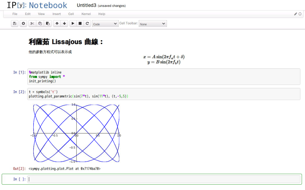
因此不易展示程式碼,故而每每以 Shell 為範。由於操作上大同小異﹐尚祈無礙矣。
【參考資料】
Plotting Module
Introduction
The plotting module allows you to make 2-dimensional and 3-dimensional plots. Presently the plots are rendered using matplotlib as a backend. It is also possible to plot 2-dimensional plots using a TextBackend if you don’t have matplotlib.
The plotting module has the following functions:
- plot: Plots 2D line plots.
- plot_parametric: Plots 2D parametric plots.
- plot_implicit: Plots 2D implicit and region plots.
- plot3d: Plots 3D plots of functions in two variables.
- plot3d_parametric_line: Plots 3D line plots, defined by a parameter.
- plot3d_parametric_surface: Plots 3D parametric surface plots.
The above functions are only for convenience and ease of use. It is possible to plot any plot by passing the corresponding Series class to Plot as argument.
【簡單範例】
pi@raspberrypi:~ $ ipython3
Python 3.4.2 (default, Oct 19 2014, 13:31:11)
Type "copyright", "credits" or "license" for more information.
IPython 2.3.0 -- An enhanced Interactive Python.
? -> Introduction and overview of IPython's features.
%quickref -> Quick reference.
help -> Python's own help system.
object? -> Details about 'object', use 'object??' for extra details.
In [1]: from sympy import *
In [2]: init_printing()
In [3]: R, r, ρ, t = symbols('R, r, ρ, t')
In [4]: x = R * ( (1 - r/R) * cos(t) + ρ/R * cos((R - r)/r * t) )
In [5]: y = R * ( (1 - r/R) * sin(t) - ρ/R * sin((R - r)/r * t) )
In [6]: x
Out[6]:
⎛ ⎛t⋅(R - r)⎞⎞
⎜ ρ⋅cos⎜─────────⎟⎟
⎜⎛ r⎞ ⎝ r ⎠⎟
R⋅⎜⎜1 - ─⎟⋅cos(t) + ────────────────⎟
⎝⎝ R⎠ R ⎠
In [7]: y
Out[7]:
⎛ ⎛t⋅(R - r)⎞⎞
⎜ ρ⋅sin⎜─────────⎟⎟
⎜⎛ r⎞ ⎝ r ⎠⎟
R⋅⎜⎜1 - ─⎟⋅sin(t) - ────────────────⎟
⎝⎝ R⎠ R ⎠
In [8]: x1 = x.subs([(R, 5), (r, 3), (ρ, 2)])
In [9]: y1 = y.subs([(R, 5), (r, 3), (ρ, 2)])
In [10]: x1
Out[10]:
⎛2⋅t⎞
2⋅cos⎜───⎟ + 2⋅cos(t)
⎝ 3 ⎠
In [11]: y1
Out[11]:
⎛2⋅t⎞
- 2⋅sin⎜───⎟ + 2⋅sin(t)
⎝ 3 ⎠
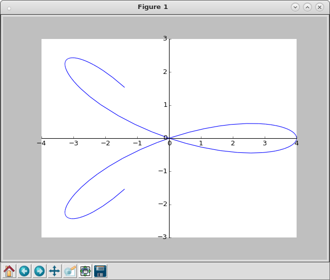
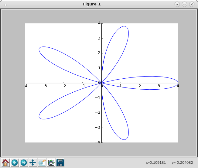
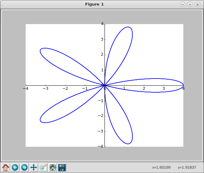
# Fig 1, Fig 2, Fig 3
In [12]: plotting.plot_parametric(x1, y1, (t, -5, 5))
Out[12]: <sympy.plotting.plot.Plot at 0x74b8cb10>
In [13]: plotting.plot_parametric(x1, y1, (t, -10, 10))
Out[13]: <sympy.plotting.plot.Plot at 0x72959d30>
In [14]: plotting.plot_parametric(x1, y1, (t, -100, 100))
Out[14]: <sympy.plotting.plot.Plot at 0x713cf990>
In [15]:
【Fig 1, Fig 2, Fig 3】