《永無休止》
無聲之歌,無言之語,此刻醉臥靜穆中。
等待………
甦醒。
號角已響起,急而又急。
人間世,
一事尚且聽未清,一事早待看分明!
………
復黎明,
萬象交織光與影。
Now Available for Download: Processing
I’m a long-time fan of Processing, a free open source programming language and development environment focused on teaching coding in the context of visual arts. It’s why I’m so excited that the latest version, Processing 3.0.1, now officially supports Raspberry Pi. Just as Sonic Pi lets you make your first sound in just one line of code, Processing lets you draw on screen with just one line of code. It’s that easy to get started. But don’t let that fool you, it’s a very powerful and flexible language and development environment.
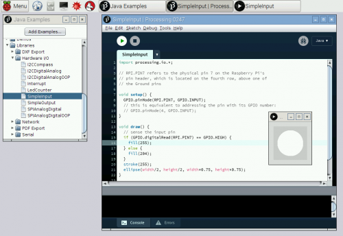
We owe a huge thank you to Gottfried Haider, who did the heavy lifting to get Processing running smoothly on the Raspberry Pi and create a hardware input/output library. That’s right, this version of Processing works with the GPIO pins right out of the box. Gottfried says:
I’m excited about having Processing on the Raspberry Pi and other low-cost desktop machines. In the last few years we’ve seen a shift away from easily accessible environments, towards concepts such as mobile platforms, specialized internet-of-things devices and cloud computing. As someone who got into programming by tinkering around with the open and readily available platforms of the time, I believe it’s important to have initiatives such Raspberry Pi and Processing, to promote software literacy and to encourage a future where computers remain a read/write medium.
───
Overview. A short introduction to the Processing software and projects from the community.
| For the past fourteen years, Processing has promoted software literacy, particularly within the visual arts, and visual literacy within technology. Initially created to serve as a software sketchbook and to teach programming fundamentals within a visual context, Processing has also evolved into a development tool for professionals. The Processing software is free and open source, and runs on the Mac, Windows, and GNU/Linux platforms.
Processing continues to be an alternative to proprietary software tools with restrictive and expensive licenses, making it accessible to schools and individual students. Its open source status encourages the community participation and collaboration that is vital to Processing’s growth. Contributors share programs, contribute code, and build libraries, tools, and modes to extend the possibilities of the software. The Processing community has written more than a hundred libraries to facilitate computer vision, data visualization, music composition, networking, 3D file exporting, and programming electronics. Processing is currently developed primarily in Boston (at Fathom Information Design), Los Angeles (at the UCLA Arts Software Studio), and New York City (at NYU’s ITP). EducationFrom the beginning, Processing was designed as a first programming language. It was inspired by earlier languages like BASIC and Logo, as well as our experiences as students and teaching visual arts foundation curricula. The same elements taught in a beginning high school or university computer science class are taught through Processing, but with a different emphasis. Processing is geared toward creating visual, interactive media, so the first programs start with drawing. Students new to programming find it incredibly satisfying to make something appear on their screen within moments of using the software. This motivating curriculum has proved successful for leading design, art, and architecture students into programming and for engaging the wider student body in general computer science classes. Processing is used in classrooms worldwide, often in art schools and visual arts programs in universities, but it’s also found frequently in high schools, computer science programs, and humanities curricula. Museums such as the Exploratorium in San Francisco use Processing to develop their exhibitions. In a National Science Foundation-sponsored survey, students in a college-level introductory computing course taught with Processing at Bryn Mawr College said they would be twice as likely to take another computer science class as the students in a class with a more traditional curriculum. The innovations in teaching through Processing have been adapted for the Khan Academy computer science tutorials, offered online for free. The tutorials begin with drawing, using most of the Processing functions for drawing. The Processing approach has also been applied to electronics through the Arduino and Wiring projects. Arduino uses a syntax inspired by that used with Processing, and continues to use a modified version of the Processing programming environment to make it easier for students to learn how to program robots and countless other electronics projects. CultureThe Processing software is used by thousands of visual designers, artists, and architects to create their works. Projects created with Processing have been featured at the Museum of Modern Art in New York, the Victoria and Albert Museum in London, the Centre Georges Pompidou in Paris, and many other prominent venues. Processing is used to create projected stage designs for dance and music performances; to generate images for music videos and film; to export images for posters, magazines, and books; and to create interactive installations in galleries, in museums, and on the street. Some prominent projects include the House of Cards video for Radiohead, the MIT Media Lab’s generative logo, and the Chronograph projected software mural for the Frank Gehry-designed New World Center in Miami. But the most important thing about Processing and culture is not high-profile results – it’s how the software has engaged a new generation of visual artists to consider programming as an essential part of their creative practice. |
………
切莫問,
來還來不及 Processing ?!
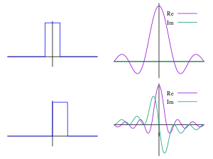
 and its Fourier transform
  , a function of frequency
  . Translation (that is, delay) in the time domain goes over to complex phase shifts in the frequency domain. In the second row is shown
  , a delayed unit pulse, beside the real and imaginary parts of the Fourier transform. The Fourier transform decomposes a function into eigenfunctions for the group of translations.
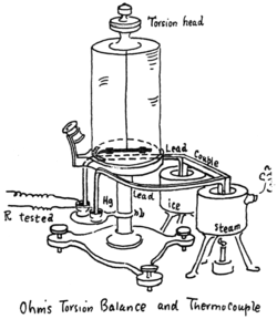


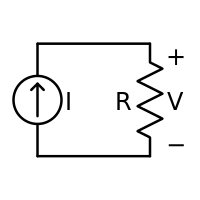
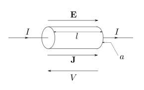

 是受測電線造成的電流差值,
 是跟實驗參數有關的係數,
 是受測電線的長度,
 是跟固定長度的載流導線有關的常數。不久之後,歐姆便發覺了這個關係式可能是不正確的。
 的函數
的函數  ,都可以用『無窮級數』表示為
 可以依下式來計算
 ,而且
,而且  是基本周期為
  時,
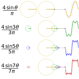
時, 係數稱之為『直流分量』,就是訊號
  時,
時, 係數是『一次諧波』頻率,隨著
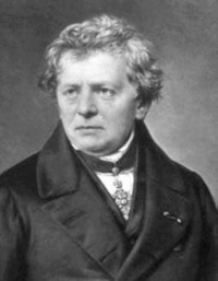
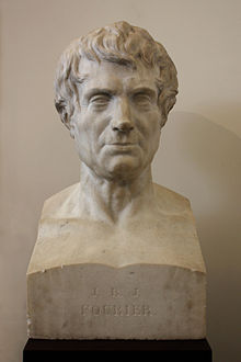
  的值,而有『二次諧波』,『三次諧波』等等。並且將之應用於『熱傳導理論』與『振動理論』;據聞他也是『溫室效應』的發現者。一八二二年傅立葉發表了《
 。
。
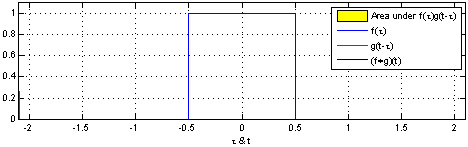
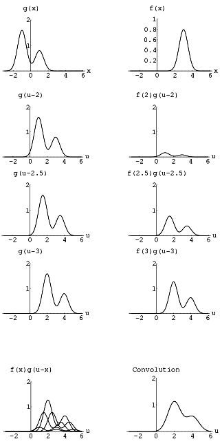
 反射,接著平移”t”,成為
 。那麼重疊部份的面積就相當於”t”處的捲積,其中橫坐標代表待積變量
 以及新函數
以及新函數 的自變量”t”。
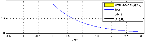
 ,
, 是
是 上的兩個可積函數,作積分:
 ,上述積分是存在的。這樣,隨著
 的不同取值,這個積分就定義了一個新函數
 ,稱為函數
,稱為函數 與
與 的摺積,記為
 。我們可以輕易驗證:
 ,並且
,並且 仍為可積函數。這就是說,把摺積代替乘法,
 空間是一個代數,甚至是
 ,不過捲積只是運算符號,理論上並不需要對函數
  有特別的限制,雖然常常要求
  一般要比
一般要比 ,這種方法稱為函數的光滑化或正則化。
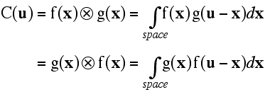
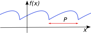


 .
. is an
is an  is a representation of a 1-periodic function.
 為『周期』的函數,自然也以
  為周期【※
為周期【※  非零正整數】,所以實數周期函數才會有最小周期值。
 以
以  為周期,
為周期,  以
以  為周期,假使
  的比值是個『有理數』,可以用『最簡分數』表示成
  。也就是說
。也就是說 
 的周期。然而周期不必是『有理數』,周期的『比值』當然也未必是『有理數』,因此
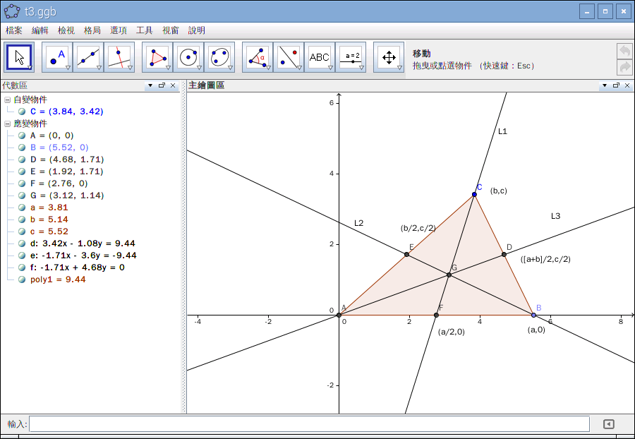
 三個參數?即使在思考過
  是此『底』之『高』,
  是此『高』距與此『底』一端的距離。我們深信這就『確定』了那個三角形。然而若再問︰如果此三角形的三個頂點用更一般的
  、
、  、
、  來表達 ,如是分明有六個參數。那麼這兩種『表述』當真是一樣的嗎?設想你在桌面上『移動』一個三角形,從此『位置』此『方位』到達彼『位置』彼『方位』,你會認為這個三角形『改變』了嗎??假使『直覺』以為『不變』,這個三角形就必得有使之『不變』的『因由』,這個『因由』不必『參照』解析幾何的『座標』而確立 。或可說它就是歐式幾何一個三角形的『定義』內涵而已。如此而言,一個『確定』的三角形,可由它的三個『邊長』來『確立』,所以六個參數補之以三個確定之邊長關係,豈非還是三個參數的耶??

 .
.
 and
and  have the same magnitude and are separated by an angle
