假使說『幾何光學』描述『光線』在不同介質裡之傳播行為︰

Geometrical optics, or ray optics, describes light propagation in terms of rays. The ray in geometric optics is an abstraction, or instrument, useful in approximating the paths along which light propagates in certain classes of circumstances.

The simplifying assumptions of geometrical optics include that light rays:

propagate in rectilinear paths as they travel in a homogeneous medium
bend, and in particular circumstances may split in two, at the interface between two dissimilar media
follow curved paths in a medium in which the refractive index changes
may be absorbed or reflected.

Geometrical optics does not account for certain optical effects such as diffraction and interference. This simplification is useful in practice; it is an excellent approximation when the wavelength is small compared to the size of structures with which the light interacts. The techniques are particularly useful in describing geometrical aspects of imaging, including optical aberrations.

───

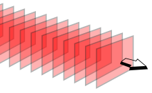
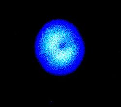
首要得先明白什麼是『光線』呢？如果將之比擬為雷射光束

LASER

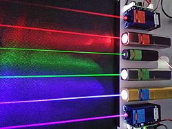
Red (660 & 635 nm), green (532 & 520 nm) and blue-violet (445 & 405 nm) lasers

或許差強人意。然而總有模模糊糊的味道。就像請人定義什麼是『質量』？若只是講『質量』就是『物質的量』，怕也難明所指的吧！此時要是援用牛頓的『第二運動定律』 $\vec F = m \cdot \vec a$ 就釐清了『質量』之明確意義為 $m = \frac{\vec F}{\vec a}$ 也！

因此『幾何光學』之基本原理 ── 費馬原理 ──

Fermat’s principle

In optics, Fermat‘s principle or the principle of least time is the principle that the path taken between two points by a ray of light is the path that can be traversed in the least time. This principle is sometimes taken as the definition of a ray of light.^[1] However, this version of the principle is not general; a more modern statement of the principle is that rays of light traverse the path of stationary optical length with respect to variations of the path.^[2] In other words, a ray of light prefers the path such that there are other paths, arbitrarily nearby on either side, along which the ray would take almost exactly the same time to traverse.

Fermat’s principle can be used to describe the properties of light rays reflected off mirrors, refracted through different media, or undergoing total internal reflection. It follows mathematically from Huygens’ principle (at the limit of small wavelength). French mathematician Pierre de Fermat’s text Analyse des réfractions exploits the technique of adequality to derive Snell’s law of refraction^[3] and the law of reflection.

Fermat’s principle has the same form as Hamilton’s principle and it is the basis of Hamiltonian optics.

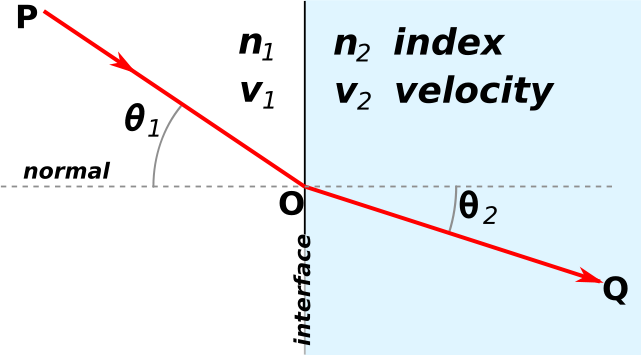
Fermat’s principle leads to Snell’s law; when the sines of the angles in the different media are in the same proportion as the propagation velocities, the time to get from P to Q is minimized.

Modern version

The time T a point of the electromagnetic wave needs to cover a path between the points A and B is given by:

T=\int_{\mathbf{t_0}}^{\mathbf{t_1}} \, dt = \frac{1}{c} \int_{\mathbf{t_0}}^{\mathbf{t_1}} \frac{c}{v} \frac{ds}{dt}\, dt = \frac{1}{c} \int_{\mathbf{A}}^{\mathbf{B}} n\, ds\

c is the speed of light in vacuum, ds an infinitesimal displacement along the ray, v = ds/dt the speed of light in a medium and n = c/v the refractive index of that medium, $t_{0}$ is the starting time (the wave front is in A), $t_{1}$ is the arrival time at B. The optical path length of a ray from a point A to a point B is defined by:

S=\int_{\mathbf{A}}^{\mathbf{B}} n\, ds\

and it is related to the travel time by S = cT. The optical path length is a purely geometrical quantity since time is not considered in its calculation. An extremum in the light travel time between two points A and B is equivalent to an extremum of the optical path length between those two points. The historical form proposed by Fermat is incomplete. A complete modern statement of the variational Fermat principle is that

the optical length of the path followed by light between two fixed points, A and B, is an extremum. The optical length is defined as the physical length multiplied by the refractive index of the material.”^[4]

In the context of calculus of variations this can be written as

\delta S= \delta\int_{\mathbf{A}}^{\mathbf{B}} n \, ds =0

In general, the refractive index is a scalar field of position in space, that is, $n=n\left(x_1,x_2,x_3\right) \$ in 3D euclidean space. Assuming now that light has a component that travels along the x₃ axis, the path of a light ray may be parametrized as $s=\left(x_1\left(x_3\right),x_2\left(x_3\right),x_3\right) \$ and

nds=n \frac{\sqrt{dx_1^2+dx_2^2+dx_3^2}}{dx_3}dx_3=n \sqrt{1+\dot{x}_1^2+\dot{x}_2^2} \ dx_3

where $\dot{x}_k=dx_k/dx_3$ . The principle of Fermat can now be written as

\delta S= \delta\int_{x_{3A}}^{x_{3B}} n\left(x_1,x_2,x_3\right) \sqrt{1+\dot{x}_1^2+\dot{x}_2^2}\, dx_3

= \delta\int_{x_{3A}}^{x_{3B}} L\left(x_1\left(x_3\right),x_2\left(x_3\right),\dot{x}_1\left(x_3\right),\dot{x}_2\left(x_3\right),x_3\right)\, dx_3=0

which has the same form as Hamilton’s principle but in which x₃ takes the role of time in classical mechanics. Function $L\left(x_1,x_2,\dot{x}_1,\dot{x}_2,x_3\right)$ is the optical Lagrangian from which the Lagrangian and Hamiltonian (as in Hamiltonian mechanics) formulations of geometrical optics may be derived.^[5]

───

也可以用來定義何謂『光線』的了！！此時再得『惠更斯原理』之光照，或可想像『光線』之行徑乎？？

$200px-Refraction_-_Huygens-Fresnel_principle.svg$

$220px-Huygens_Refracted_Waves$

$200px-Refraction_on_an_aperture_-_Huygens-Fresnel_principle.svg$

$Circular_Aperture_Fresnel_Diffraction_high_res$

惠更斯原理
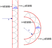
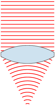
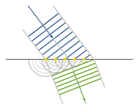
在『波前』wavefront 上的每一個點都可以將它看成是產生『球面次波』Spherical secondary waves 的『點波源』，而在這『之後』任何時刻的『波前』則可看作是這一些『相同相位子波』的『包絡』Envlope 『線』或者『面』。

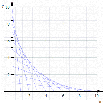
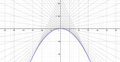
那麼什麼是『包絡』的呢？從幾何學上講，一個『曲線族』的『包絡線』與該曲線族中的每一條曲線都『相切』tangent to 於某一點。一七三四年法國數學家亞歷克西斯‧克勞德‧克萊羅 Alexis Claude de Clairault 提出 $y(x)=x\frac{dy}{dx}+f\left(\frac{dy}{dx}\right)$ 方程式。如果將該方程式對變數 $x$ 再次作『微分』得到 $0=\left(x+f'\left(\frac{dy}{dx}\right)\right)\frac{d^2 y}{dx^2}$ ，因此 $0=\frac{d^2 y}{dx^2}$ 或者 $0=x+f'\left(\frac{dy}{dx}\right)$ 。假使 $0=\frac{d^2 y}{dx^2}$ ，那麼 $\frac{dy}{dx} = C$ 是一個『常數』，將之代入原方程式得到『曲線族』 $y(x)=Cx+f(C)$ 的一般解。如果 $0=x+f'\left(\frac{dy}{dx}\right)$ ，它的解是上述曲線族的『包絡線』。舉例而言，下圖是 $f(p) = p^2$ 的圖示

其次『波前』的形狀可以被經過的『光學系統』所改變；而『相位相同』是講在 $t$ 時間的波前『次波』都經過了『相同』的『時距』 $\Delta t$ ，形成了 $t^{'} = t + \Delta t$ 新的波前。

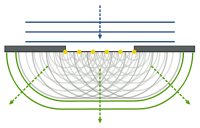
藉著這原理，惠更斯給出了波的『直線傳播』與『球面傳播』的『定性』解釋，並且推導出了『反射定律』與『折射定律』。但是他卻不能解釋，為什麼當光波遇到『銳邊』、『小孔』或『狹縫』時，會偏離了直線傳播，也就是說會發生『繞射』現象。除此之外『惠更斯原理』假設了『次波』只會朝著『行進方向』傳播；然而他並沒有解釋為什麼它們不可以朝反方向傳播的呢？

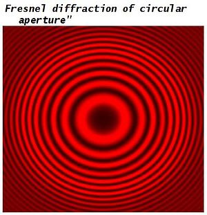
法國物理學家奧古斯丁‧菲涅耳 Augustin Fresnel ，是『波動光學理論』的主要創建者之一，在惠更斯原理的基礎上假設這些『次波會彼此發生干涉』，這就是現今所稱的『惠更斯‧菲涅耳原理』，是『惠更斯原理』與『干涉原理』的開花結果。一八一八年菲涅耳將他的論文提交給法蘭西學術院的評委會。評委會的會員西莫恩‧德尼‧帕松 Siméon Denis Poisson 認為假使菲涅耳的理論成立，那麼將光波照射於一小塊圓形擋板時，所形成的陰影之中央必定會有一個亮斑，因此他推斷這理論不正確。同時與會的弗朗索瓦‧讓‧多米尼克‧阿拉戈 François Jean Dominique Arago 親自動手做了這個實驗，結果與預測相符，證實了菲涅耳原理的正確無誤。這實驗是支持光波動說的強有力的證據，與楊氏的雙縫實驗共同反駁了牛頓主導的光粒子說。

─── 摘自《【Sonic π】聲波之傳播原理︰原理篇《二》》

那個『波前』的『法向量』正標示『光線』之流向也！！

在此就讓我們借著

變分法

變分法是處理泛函的數學領域，和處理函數的普通微積分相對。譬如，這樣的泛函可以通過未知函數的積分和它的導數來構造。變分法最終尋求的是極值函數：它們使得泛函取得極大或極小值。有些曲線上的經典問題採用這種形式表達：一個例子是最速降線，在重力作用下一個粒子沿著該路徑可以在最短時間從點A到達不直接在它底下的一點B。在所有從A到B的曲線中必須極小化代表下降時間的表達式。

變分法的關鍵定理是歐拉－拉格朗日方程。它對應於泛函的臨界點。在尋找函數的極大和極小值時，在一個解附近的微小變化的分析給出一階的一個近似。它不能分辨是找到了最大值或者最小值（或者都不是）。

變分法在理論物理中非常重要：在拉格朗日力學中，以及在最小作用量原理在量子力學的應用中。變分法提供了有限元方法的數學基礎，它是求解邊界值問題的強力工具。它們也在材料學中研究材料平衡中大量使用。而在純數學中的例子有，黎曼在調和函數中使用狄利克雷原理。

同樣的材料可以出現在不同的標題中，例如希爾伯特空間技術，莫爾斯理論，或者辛幾何。變分一詞用於所有極值泛函問題。微分幾何中的測地線的研究是很顯然的變分性質的領域。極小曲面（肥皂泡）上也有很多研究工作，稱為普拉托問題。

───

用『任意鄰近函式』 $\delta x(t) = \epsilon \cdot \eta (t)$ 的概念

Euler–Lagrange equation

Main article: Euler–Lagrange equation

Finding the extrema of functionals is similar to finding the maxima and minima of functions. The maxima and minima of a function may be located by finding the points where its derivative vanishes (i.e., is equal to zero). The extrema of functionals may be obtained by finding functions where the functional derivative is equal to zero. This leads to solving the associated Euler–Lagrange equation.^{[Note 3]}

Consider the functional

J[y] = \int_{x_1}^{x_2} L(x,y(x),y'(x))\, dx \, .

where

x 1, x 2

are constants,

y (x)

is twice continuously differentiable,

y'(x) = dy / dx

L (x, y (x), y'(x))

is twice continuously differentiable with respect to its arguments

x, y, y'

If the functional $J [y]$ attains a local minimum at $f,$ and $η (x)$ is an arbitrary function that has at least one derivative and vanishes at the endpoints $x 1$ and $x 2,$ then for any number $ε$ close to 0,

J[f] \le J[f + \varepsilon \eta] \, .

The term $εη$ is called the variation of the function $f$ and is denoted by $δf .$ ^[11]

Substituting $f + εη$ for $y$ in the functional $J [y] ,$ the result is a function of $ε$ ,

\Phi(\varepsilon) = J[f+\varepsilon\eta] \, .

Since the functional $J [y]$ has a minimum for $y = f,$ the function $Φ(ε)$ has a minimum at $ε = 0$ and thus,^{[Note 4]}

\Phi'(0) \equiv \left.\frac{d\Phi}{d\varepsilon}\right|_{\varepsilon = 0} = \int_{x_1}^{x_2} \left.\frac{dL}{d\varepsilon}\right|_{\varepsilon = 0} dx = 0 \, .

Taking the total derivative of $L [x, y, y'] ,$ where $y = f + ε η$ and $y' = f' + ε η'$ are functions of $ε$ but $x$ is not,

\frac{dL}{d\varepsilon}=\frac{\partial L}{\partial y}\frac{dy}{d\varepsilon} + \frac{\partial L}{\partial y'}\frac{dy'}{d\varepsilon}

and since $dy / dε = η$ and $dy'/ dε = η’$ ,

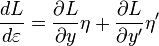\frac{dL}{d\varepsilon}=\frac{\partial L}{\partial y}\eta + \frac{\partial L}{\partial y'}\eta'

Therefore,

\text{[math]}

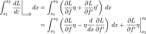
where $L [x, y, y'] \to L [x, f, f']$ when ε = 0 and we have used integration by parts. The last term vanishes because $η = 0$ at $x 1$ and $x 2$ by definition. Also, as previously mentioned the left side of the equation is zero so that

\int_{x_1}^{x_2} \eta \left(\frac{\partial L}{\partial f} - \frac{d}{dx}\frac{\partial L}{\partial f'} \right) \, dx = 0 \, .

According to the fundamental lemma of calculus of variations, the part of the integrand in parentheses is zero, i.e.

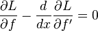
\frac{\part L}{\part f} -\frac{d}{dx} \frac{\part L}{\part f'}=0

which is called the Euler–Lagrange equation. The left hand side of this equation is called the functional derivative of $J [f]$ and is denoted $δJ / δf (x) .$

In general this gives a second-order ordinary differential equation which can be solved to obtain the extremal function $f (x) .$ The Euler–Lagrange equation is a necessary, but not sufficient, condition for an extremum $J [f]$ . A sufficient condition for a minimum is given in the section Variations and sufficient condition for a minimum.

─── 摘自《W!o+ 的《小伶鼬工坊演義》︰神經網絡【轉折點】四中》

以『在均勻介質中，光走直線。』為例。對比

【紙筆計算】

Example

In order to illustrate this process, consider the problem of finding the extremal function $y = f (x) ,$ which is the shortest curve that connects two points $(x 1, y 1)$ and $(x 2, y 2) .$ The arc length of the curve is given by

A[y]=\int _{x_{1}}^{x_{2}}{\sqrt {1+[y'(x)]^{2}}}\,dx\,,

with

y\,'(x)={\frac {dy}{dx}}\,,\ \ y_{1}=f(x_{1})\,,\ \ y_{2}=f(x_{2})\,.

The Euler–Lagrange equation will now be used to find the extremal function $f (x)$ that minimizes the functional $A [y] .$

{\frac {\partial L}{\partial f}}-{\frac {d}{dx}}{\frac {\partial L}{\partial f'}}=0

with

L={\sqrt {1+[f'(x)]^{2}}}\,.

Since $f$ does not appear explicitly in $L,$ the first term in the Euler–Lagrange equation vanishes for all $f (x)$ and thus,

{\frac {d}{dx}}{\frac {\partial L}{\partial f'}}=0\,.

Substituting for $L$ and taking the partial derivative,

{\frac {d}{dx}}\ {\frac {f'(x)}{\sqrt {1+[f'(x)]^{2}}}}\ =0\,.

Taking the derivative $d/dx$ and simplifying gives,

{\frac {d^{2}f}{dx^{2}}}\ \cdot \ {\frac {1}{\left[{\sqrt {1+[f'(x)]^{2}}}\ \right]^{3}}}=0\,,

and because $1+[f ' (x)] 2$ is non-zero,

{\frac {d^{2}f}{dx^{2}}}=0\,,

which implies that the shortest curve that connects two points $(x 1, y 1)$ and $(x 2, y 2)$ is

f(x)=mx+b\qquad {\text{with}}\ \ m={\frac {y_{2}-y_{1}}{x_{2}-x_{1}}}\quad {\text{and}}\quad b={\frac {x_{2}y_{1}-x_{1}y_{2}}{x_{2}-x_{1}}}

and we have thus found the extremal function $f (x)$ that minimizes the functional $A [y]$ so that $A [f]$ is a minimum. Note that $y = f (x)$ is the equation for a straight line, in other words, the shortest distance between two points is a straight line.^{[Note 5]}

───

與

【SymPy 符號運算】

pi@raspberrypi:~ $ python3
Python 3.4.2 (default, Oct 19 2014, 13:31:11) 
[GCC 4.9.1] on linux
Type "help", "copyright", "credits" or "license" for more information.
>>> from sympy import *
>>> init_printing()
>>> y = Function('y')
>>> x = Symbol('x')
>>> L = sqrt(1 + (y(x).diff(x))**2)
>>> L
     _________________
    ╱           2     
   ╱  ⎛d       ⎞      
  ╱   ⎜──(y(x))⎟  + 1 
╲╱    ⎝dx      ⎠      
>>> E = euler_equations(L, y(x),x)
>>> E
⎡ ⎛                2  ⎞               ⎤
⎢ ⎜      ⎛d       ⎞   ⎟               ⎥
⎢ ⎜      ⎜──(y(x))⎟   ⎟   2           ⎥
⎢ ⎜      ⎝dx      ⎠   ⎟  d            ⎥
⎢-⎜1 - ───────────────⎟⋅───(y(x))     ⎥
⎢ ⎜              2    ⎟   2           ⎥
⎢ ⎜    ⎛d       ⎞     ⎟ dx            ⎥
⎢ ⎜    ⎜──(y(x))⎟  + 1⎟               ⎥
⎢ ⎝    ⎝dx      ⎠     ⎠               ⎥
⎢───────────────────────────────── = 0⎥
⎢           _________________         ⎥
⎢          ╱           2              ⎥
⎢         ╱  ⎛d       ⎞               ⎥
⎢        ╱   ⎜──(y(x))⎟  + 1          ⎥
⎣      ╲╱    ⎝dx      ⎠               ⎦

>>> dsolve(y(x).diff(x,x))
y(x) = C₁ + C₂⋅x
>>>

之差異。

日	一	二	三	四	五	六
« 4 月
	1	2	3	4	5	6
7	8	9	10	11	12	13
14	15	16	17	18	19	20
21	22	23	24	25	26	27
28	29	30

FreeSandal

光的世界︰幾何光學一

Fermat’s principle

Modern version

變分法

Euler–Lagrange equation

Example

輕。鬆。學。部落客