什麼是事物的『特徵』呢?為什麼它的『提取方法』很重要?維基百科詞條這麼說︰
Feature extraction
In machine learning, pattern recognition and in image processing, feature extraction starts from an initial set of measured data and builds derived values (features) intended to be informative and non-redundant, facilitating the subsequent learning and generalization steps, and in some cases leading to better human interpretations. Feature extraction is related to dimensionality reduction.
When the input data to an algorithm is too large to be processed and it is suspected to be redundant (e.g. the same measurement in both feet and meters, or the repetitiveness of images presented as pixels), then it can be transformed into a reduced set of features (also named a features vector). This process is called feature selection. The selected features are expected to contain the relevant information from the input data, so that the desired task can be performed by using this reduced representation instead of the complete initial data.
───
假使考慮如何『定義』事物耶?也許『特徵』就是『界定性徵』,可以用來『區分』相異的東西!所以人們自然懂得『汪星人』不同於『喵星人』的也!!
於是乎好奇那『聲音』本有『調子』,可以用
Cepstrum
A cepstrum (/ˈkɛpstrəmˈˌˈsɛpstrəmˈ/) is the result of taking the Inverse Fourier transform (IFT) of the logarithm of the estimated spectrum of a signal. It may be pronounced in the two ways given, the second having the advantage of avoiding confusion with ‘kepstrum’ which also exists (see below). There is a complex cepstrum, a real cepstrum, a power cepstrum, and a phase cepstrum. The power cepstrum in particular finds applications in the analysis of human speech.
The name “cepstrum” was derived by reversing the first four letters of “spectrum”. Operations on cepstra are labelled quefrency analysis (aka quefrency alanysis[1]), liftering, or cepstral analysis.

Steps in forming cepstrum from time history
───
來探討。那麼『圖象』可有『調子』乎?!能否依樣畫葫蘆來研究的呢!?不管『笨鳥先飛』、『菜鳥忘飛』、『老鳥已飛』……… 科技史裡滿載『傻問題』之『大成就』矣!!??何不就效法一下嘛??!!
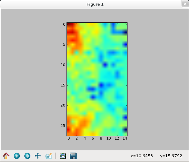
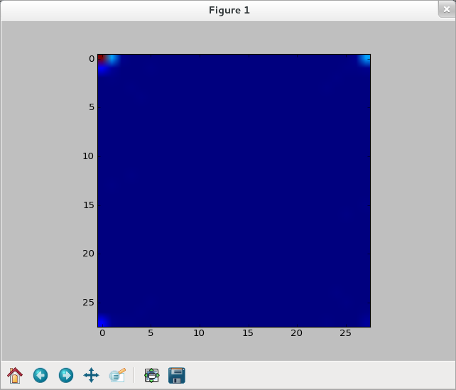
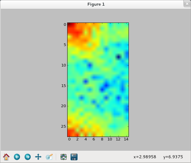
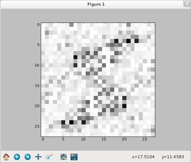
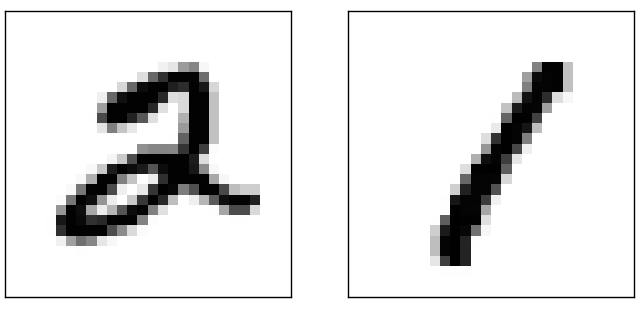
【還是用五】
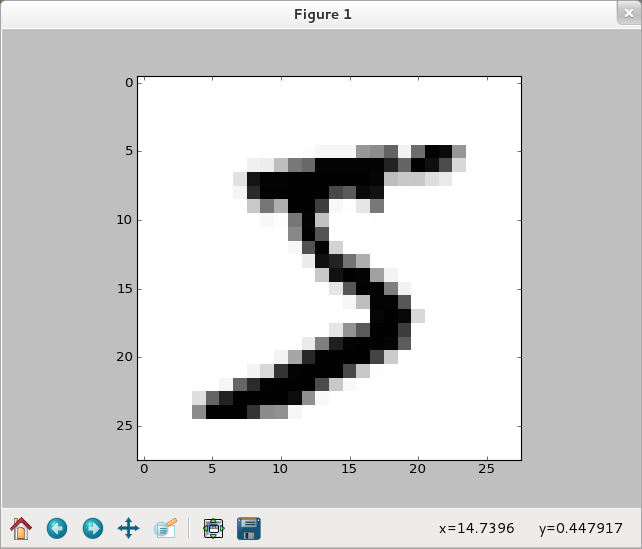
>>> img = training_data[0][0].reshape(28,28)
>>> f_img = network.np.fft.rfft2(img)
>>> logp_img = 2*network.np.log(network.np.abs(f_img))
>>> plt.imshow(logp_img)
<matplotlib.image.AxesImage object at 0x51af290>
>>> plt.show()
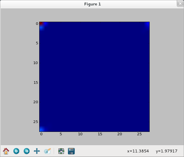
>>> ilogpf_img = network.np.fft.irfft2(logp_img)
>>> cf_img = network.np.abs(ilogpf_img)**2
>>> plt.imshow(cf_img)
<matplotlib.image.AxesImage object at 0x51d1050>
>>> plt.show()
【依舊選零】
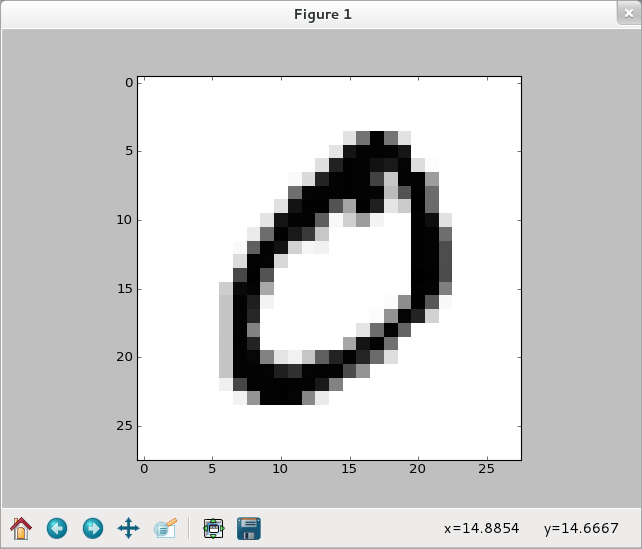
>>> img1 = training_data[1][0].reshape(28,28)
>>> f_img1 = network.np.fft.rfft2(img1)
>>> logp_img1 = 2*network.np.log(network.np.abs(f_img1))
>>> plt.imshow(logp_img1)
<matplotlib.image.AxesImage object at 0x5091e50>
>>> plt.show()
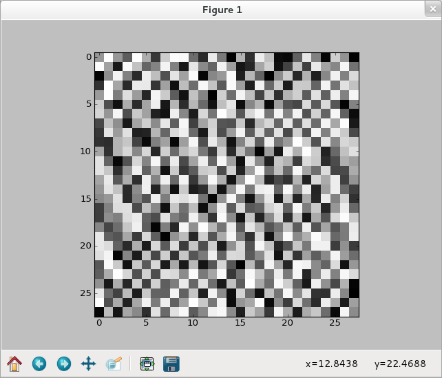
>>> ilogpf_img1 = network.np.fft.irfft2(logp_img1)
>>> cf_img1 = network.np.abs(ilogpf_img1)**2
>>> plt.imshow(cf_img1)
<matplotlib.image.AxesImage object at 0x51b9b50>
>>> plt.show()
>>>
【參考資料】
Discrete Fourier Transform (numpy.fft)
Standard FFTs
| fft(a[, n, axis, norm]) | Compute the one-dimensional discrete Fourier Transform. |
| ifft(a[, n, axis, norm]) | Compute the one-dimensional inverse discrete Fourier Transform. |
| fft2(a[, s, axes, norm]) | Compute the 2-dimensional discrete Fourier Transform This function computes the n-dimensional discrete Fourier Transform over any axes in an M-dimensional array by means of the Fast Fourier Transform (FFT). |
| ifft2(a[, s, axes, norm]) | Compute the 2-dimensional inverse discrete Fourier Transform. |
| fftn(a[, s, axes, norm]) | Compute the N-dimensional discrete Fourier Transform. |
| ifftn(a[, s, axes, norm]) | Compute the N-dimensional inverse discrete Fourier Transform. |
Real FFTs
| rfft(a[, n, axis, norm]) | Compute the one-dimensional discrete Fourier Transform for real input. |
| irfft(a[, n, axis, norm]) | Compute the inverse of the n-point DFT for real input. |
| rfft2(a[, s, axes, norm]) | Compute the 2-dimensional FFT of a real array. |
| irfft2(a[, s, axes, norm]) | Compute the 2-dimensional inverse FFT of a real array. |
| rfftn(a[, s, axes, norm]) | Compute the N-dimensional discrete Fourier Transform for real input. |
| irfftn(a[, s, axes, norm]) | Compute the inverse of the N-dimensional FFT of real input. |
Hermitian FFTs
| hfft(a[, n, axis, norm]) | Compute the FFT of a signal which has Hermitian symmetry (real spectrum). |
| ihfft(a[, n, axis, norm]) | Compute the inverse FFT of a signal which has Hermitian symmetry. |
Helper routines
| fftfreq(n[, d]) | Return the Discrete Fourier Transform sample frequencies. |
| rfftfreq(n[, d]) | Return the Discrete Fourier Transform sample frequencies (for usage with rfft, irfft). |
| fftshift(x[, axes]) | Shift the zero-frequency component to the center of the spectrum. |
| ifftshift(x[, axes]) | The inverse of fftshift. |
Background information
Fourier analysis is fundamentally a method for expressing a function as a sum of periodic components, and for recovering the function from those components. When both the function and its Fourier transform are replaced with discretized counterparts, it is called the discrete Fourier transform (DFT). The DFT has become a mainstay of numerical computing in part because of a very fast algorithm for computing it, called the Fast Fourier Transform (FFT), which was known to Gauss (1805) and was brought to light in its current form by Cooley and Tukey [CT]. Press et al. [NR] provide an accessible introduction to Fourier analysis and its applications.
Because the discrete Fourier transform separates its input into components that contribute at discrete frequencies, it has a great number of applications in digital signal processing, e.g., for filtering, and in this context the discretized input to the transform is customarily referred to as a signal, which exists in the time domain. The output is called a spectrum or transform and exists in the frequency domain.
Implementation details
There are many ways to define the DFT, varying in the sign of the exponent, normalization, etc. In this implementation, the DFT is defined as

The DFT is in general defined for complex inputs and outputs, and a single-frequency component at linear frequency  is represented by a complex exponential
  , where
  is the sampling interval.
The values in the result follow so-called “standard” order: If A = fft(a, n), then A[0] contains the zero-frequency term (the mean of the signal), which is always purely real for real inputs. Then A[1:n/2] contains the positive-frequency terms, and A[n/2+1:] contains the negative-frequency terms, in order of decreasingly negative frequency. For an even number of input points, A[n/2] represents both positive and negative Nyquist frequency, and is also purely real for real input. For an odd number of input points, A[(n-1)/2] contains the largest positive frequency, while A[(n+1)/2] contains the largest negative frequency. The routine np.fft.fftfreq(n) returns an array giving the frequencies of corresponding elements in the output. The routine np.fft.fftshift(A) shifts transforms and their frequencies to put the zero-frequency components in the middle, and np.fft.ifftshift(A) undoes that shift.
When the input a is a time-domain signal and A = fft(a), np.abs(A) is its amplitude spectrum and np.abs(A)**2 is its power spectrum. The phase spectrum is obtained by np.angle(A).
The inverse DFT is defined as

It differs from the forward transform by the sign of the exponential argument and the default normalization by  .
.
───
竟然會看起來很像??似乎又有點不一樣!!到底該說是『行』還是『不行』的呀???
 ,降低到
,降低到  ,其中
,其中  為資料大小。
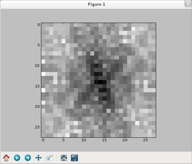
 ,它是
,它是 的一個
的一個 。任一複數都可表達為
 ,其中
,其中 及
及 皆為實數,分別稱為複數之「實部」和「虛部」。


![python mnist_average_darkness.py Baseline classifier using average darkness of image. 2225 of 10000 values correct.</pre> <span style="color: #666699;">若問什麼是『Support Vector Machine』 SVM ,維基百科詞條這麼說︰</span> <h1 id="firstHeading" class="firstHeading" lang="zh-TW"><span style="color: #666699;"><a style="color: #666699;" href="https://zh.wikipedia.org/zh-tw/%E6%94%AF%E6%8C%81%E5%90%91%E9%87%8F%E6%9C%BA">支持向量機</a></span></h1> <span style="color: #808080;"><b>支持向量機</b>(<span class="LangWithName">英語:<span lang="en"><b>Support Vector Machine</b></span></span>,常簡稱為<b>SVM</b>)是一種<a style="color: #808080;" title="監督式學習" href="https://zh.wikipedia.org/wiki/%E7%9B%A3%E7%9D%A3%E5%BC%8F%E5%AD%B8%E7%BF%92">監督式學習</a>的方法,可廣泛地應用於<a class="mw-redirect" style="color: #808080;" title="統計分類" href="https://zh.wikipedia.org/wiki/%E7%BB%9F%E8%AE%A1%E5%88%86%E7%B1%BB">統計分類</a>以及<a class="mw-redirect" style="color: #808080;" title="回歸分析" href="https://zh.wikipedia.org/wiki/%E5%9B%9E%E5%BD%92%E5%88%86%E6%9E%90">回歸分析</a>。</span> <span style="color: #808080;">支持向量機屬於一般化<a style="color: #808080;" title="線性分類器" href="https://zh.wikipedia.org/wiki/%E7%BA%BF%E6%80%A7%E5%88%86%E7%B1%BB%E5%99%A8">線性分類器</a>,也可以被認為是<a class="new" style="color: #808080;" title="提克洛夫規範化(頁面不存在)" href="https://zh.wikipedia.org/w/index.php?title=%E6%8F%90%E5%85%8B%E6%B4%9B%E5%A4%AB%E8%A7%84%E8%8C%83%E5%8C%96&action=edit&redlink=1">提克洛夫規範化</a>(Tikhonov Regularization)方法的一個特例。這族分類器的特點是他們能夠同時最小化經驗誤差與最大化幾何邊緣區,因此支持向量機也被稱為最大邊緣區分類器。</span> <h2><span id=".E4.BB.8B.E7.BB.8D" class="mw-headline" style="color: #808080;">介紹</span></h2> <span style="color: #808080;">支持向量機建構一個或多個<a style="color: #808080;" title="維度" href="https://zh.wikipedia.org/wiki/%E7%B6%AD%E5%BA%A6">高維</a>(甚至是無限多維)的<a style="color: #808080;" title="超平面" href="https://zh.wikipedia.org/wiki/%E8%B6%85%E5%B9%B3%E9%9D%A2">超平面</a>來<a class="mw-redirect" style="color: #808080;" title="統計分類" href="https://zh.wikipedia.org/wiki/%E7%BB%9F%E8%AE%A1%E5%88%86%E7%B1%BB">分類</a>資料點,這個超平面即為分類邊界。直觀來說,好的分類邊界要距離最近的訓練資料點越遠越好,因為這樣可以減低分類器的<a style="color: #808080;" title="泛化誤差" href="https://zh.wikipedia.org/wiki/%E6%B3%9B%E5%8C%96%E8%AF%AF%E5%B7%AE">泛化誤差</a>。在支持向量機中,分類邊界與最近的訓練資料點之間的距離稱為<b>間隔</b>(margin);支持向量機的目標即為找出間隔最大的超平面來作為分類邊界。</span> <span style="color: #808080;">支持向量機的<b>支持向量</b>指的就是與分類邊界距離最近的訓練資料點。從支持向量機的最佳化問題可以推導出一個重要性質:支持向量機的分類邊界可由支持向量決定,而與其他資料點無關。這也是它們稱為「支持向量」的原因。</span> <span style="color: #808080;">我們通常希望分類的過程是一個<a style="color: #808080;" title="機器學習" href="https://zh.wikipedia.org/wiki/%E6%9C%BA%E5%99%A8%E5%AD%A6%E4%B9%A0">機器學習</a>的過程。這些數據點並不需要是<img class="mwe-math-fallback-image-inline tex" src="https://upload.wikimedia.org/math/a/1/f/a1fd49f304c1094efe3fda098d5eaa5f.png" alt="\mathbb{R}^2" />中的點,而可以是任意<img class="mwe-math-fallback-image-inline tex" src="https://upload.wikimedia.org/math/5/6/e/56ef1cb9c0683de06f05e34c0bd42537.png" alt="\mathbb{R}^p" />(統計學符號)中或者<img class="mwe-math-fallback-image-inline tex" src="https://upload.wikimedia.org/math/3/0/c/30c28f76ef7517dbd19df4d4c683dbe6.png" alt="\mathbb{R}^n" />(計算機科學符號)的點。我們希望能夠把這些點通過一個n-1維的<a style="color: #808080;" title="超平面" href="https://zh.wikipedia.org/wiki/%E8%B6%85%E5%B9%B3%E9%9D%A2">超平面</a>分開,通常這個被稱為<a style="color: #808080;" title="線性分類器" href="https://zh.wikipedia.org/wiki/%E7%BA%BF%E6%80%A7%E5%88%86%E7%B1%BB%E5%99%A8">線性分類器</a>。有很多分類器都符合這個要求,但是我們還希望找到分類最佳的平面,即使得屬於兩個不同類的數據點間隔最大的那個面,該面亦稱為<b>最大間隔超平面</b>。如果能夠找到這個面,那麼這個分類器就稱為最大間隔分類器。</span> <img class="alignnone size-full wp-image-52429" src="http://www.freesandal.org/wp-content/uploads/512px-Classifier.svg.png" alt="512px-Classifier.svg" width="512" height="512" /> <span style="color: #999999;">有很多個分類器(超平面)可以把數據分開,但是只有一個能夠達到最大間隔。</span> <h3><span id=".E9.97.AE.E9.A2.98.E5.AE.9A.E4.B9.89" class="mw-headline" style="color: #808080;">問題定義</span></h3> <span style="color: #808080;">我們考慮以下形式的<img class="mwe-math-fallback-image-inline tex" src="https://upload.wikimedia.org/math/7/b/8/7b8b965ad4bca0e41ab51de7b31363a1.png" alt="n" />點測試集<img class="mwe-math-fallback-image-inline tex" src="https://upload.wikimedia.org/math/0/e/4/0e4c3d09377b2eaa4053d184400c6616.png" alt="\mathcal{D}" />:</span> <dl><dd><span style="color: #808080;"><img class="mwe-math-fallback-image-inline tex" src="https://upload.wikimedia.org/math/c/4/e/c4e8b459adf0dce2044dc139d4a4f313.png" alt="\mathcal{D}=\{(\mathbf{x}_i,y_i)| \mathbf{x}_i \in \mathbb{R}^p, y_i \in \{-1,1\} \}_{i=1}^{n}" /></span></dd></dl><span style="color: #808080;">其中<img class="mwe-math-fallback-image-inline tex" src="https://upload.wikimedia.org/math/1/8/d/18daef71b5d25ce76b8628a81e4fc76b.png" alt="y_i" />是<img class="mwe-math-fallback-image-inline tex" src="https://upload.wikimedia.org/math/6/b/b/6bb61e3b7bce0931da574d19d1d82c88.png" alt="-1" />或者<img class="mwe-math-fallback-image-inline tex" src="https://upload.wikimedia.org/math/c/4/c/c4ca4238a0b923820dcc509a6f75849b.png" alt="1" />。</span> <span style="color: #808080;">超平面的數學形式可以寫作:</span> <dl><dd><span style="color: #808080;"><img class="mwe-math-fallback-image-inline tex" src="https://upload.wikimedia.org/math/1/2/d/12dc86d8a0deebb51533508a7f027ca3.png" alt="\mathbf{w}\cdot\mathbf{x} - b=0" />。</span></dd></dl><span style="color: #808080;">其中<img class="mwe-math-fallback-image-inline tex" src="https://upload.wikimedia.org/math/3/c/6/3c66d9170d4c3fb75456e1a9fc6ead37.png" alt="\mathbf{x}" />是超平面上的點,<img class="mwe-math-fallback-image-inline tex" src="https://upload.wikimedia.org/math/2/c/5/2c5a3544056eab0411512e37fedea46d.png" alt="\mathbf{w}" />是垂直於超平面的向量。</span> <span style="color: #808080;">根據幾何知識,我們知道<img class="mwe-math-fallback-image-inline tex" src="https://upload.wikimedia.org/math/2/c/5/2c5a3544056eab0411512e37fedea46d.png" alt="\mathbf{w}" />向量垂直於分類超平面。加入位移<b>b</b>的目的是增加間隔。如果沒有<i>b</i>的話,那超平面將不得不通過原點,限制了這個方法的靈活性。</span> <span style="color: #808080;">由於我們要求最大間隔,因此我們需要知道支持向量以及(與最佳超平面)平行的並且離支持向量最近的超平面。我們可以看到這些平行超平面可以由方程族:</span> <dl><dd><span style="color: #808080;"><img class="mwe-math-fallback-image-inline tex" src="https://upload.wikimedia.org/math/d/2/9/d29858140149355ee18a76f035dec13a.png" alt="\mathbf{w}\cdot\mathbf{x} - b=1" /></span></dd></dl><span style="color: #808080;">或是</span> <dl><dd><span style="color: #808080;"><img class="mwe-math-fallback-image-inline tex" src="https://upload.wikimedia.org/math/1/5/b/15b2c2325ec495f37069bd03a137fa1f.png" alt="\mathbf{w}\cdot\mathbf{x} - b=-1" /></span></dd></dl><span style="color: #808080;">來表示,由於<img class="mwe-math-fallback-image-inline tex" src="https://upload.wikimedia.org/math/2/c/5/2c5a3544056eab0411512e37fedea46d.png" alt="\mathbf{w}" />只是超平面的法向量,長度未定,是一個變量,所以等式右邊的1和-1隻是為計算方便而取的常量,其他常量只要互為相反數亦可。</span> <span style="color: #808080;">如果這些訓練數據是線性可分的,那就可以找到這樣兩個超平面,在它們之間沒有任何樣本點並且這兩個超平面之間的距離也最大。通過幾何不難得到這兩個超平面之間的距離是2/|<i><b>w</b></i>|,因此我們需要最小化 |<i><b>w</b></i>|。同時為了使得樣本數據點都在超平面的間隔區以外,我們需要保證對於所有的<img class="mwe-math-fallback-image-inline tex" src="https://upload.wikimedia.org/math/8/6/5/865c0c0b4ab0e063e5caa3387c1a8741.png" alt="i" />滿足其中的一個條件:</span> <dl><dd><span style="color: #808080;"><img class="mwe-math-fallback-image-inline tex" src="https://upload.wikimedia.org/math/2/b/b/2bba01aaa6db12e99e73287bebf2cad9.png" alt="\mathbf{w}\cdot\mathbf{x_i} - b \ge 1\qquad\mathrm{}" /></span></dd></dl><span style="color: #808080;">或是</span> <dl><dd><span style="color: #808080;"><img class="mwe-math-fallback-image-inline tex" src="https://upload.wikimedia.org/math/f/f/6/ff60a9e0368a9230d64b4a0bd593d038.png" alt="\mathbf{w}\cdot\mathbf{x_i} - b \le -1\qquad\mathrm{}" /></span></dd></dl><span style="color: #808080;">這兩個式子可以寫作:</span> <dl><dd><span style="color: #808080;"><img class="mwe-math-fallback-image-inline tex" src="https://upload.wikimedia.org/math/b/5/9/b593983ab96553a2b4ad3219e3107fe0.png" alt="y_i(\mathbf{w}\cdot\mathbf{x_i} - b) \ge 1, \quad 1 \le i \le n.\qquad\qquad (1)" /></span></dd></dl> <h3><img class="alignnone size-full wp-image-52432" src="http://www.freesandal.org/wp-content/uploads/SVM_margins.png" alt="SVM_margins" width="740" height="903" /></h3> <span style="color: #999999;">設樣本屬於兩個類,用該樣本訓練svm得到的最大間隔超平面。在超平面上的樣本點也稱為支持向量。</span> <h3><span id=".E5.8E.9F.E5.9E.8B" class="mw-headline" style="color: #808080;">原型</span></h3> <span style="color: #808080;">現在尋找最佳超平面這個問題就變成了在(1)這個約束條件下最小化|<i><b>w</b></i>|.這是一個<a style="color: #808080;" title="二次規劃" href="https://zh.wikipedia.org/wiki/%E4%BA%8C%E6%AC%A1%E8%A7%84%E5%88%92">二次規劃</a>(QPquadratic programming)<a style="color: #808080;" title="最優化" href="https://zh.wikipedia.org/wiki/%E6%9C%80%E4%BC%98%E5%8C%96">最優化</a>中的問題。</span> <span style="color: #808080;">更清楚的表示:</span> <dl><dd><span style="color: #808080;"><img class="mwe-math-fallback-image-inline tex" src="https://upload.wikimedia.org/math/9/3/7/9376db80f8e3c1044354b455431b71ae.png" alt="\arg\min_{\mathbf{w},b}{||\mathbf{w}||^2\over2}" />,滿足<img class="mwe-math-fallback-image-inline tex" src="https://upload.wikimedia.org/math/1/6/b/16bf786b49cd616f713b9414a50b40e5.png" alt="y_i(\mathbf{w}\cdot\mathbf{x_i} - b) \ge 1" /></span></dd></dl><span style="color: #808080;">其中<img class="mwe-math-fallback-image-inline tex" src="https://upload.wikimedia.org/math/4/d/e/4de0f8ba6b80f41fe9152789af172da1.png" alt="i = 1, \dots, n" />。 1/2因子是為了數學上表達的方便加上的。</span> <span style="color: #808080;">解如上約束問題,通常的想法可能是使用非負<a style="color: #808080;" title="拉格朗日乘數" href="https://zh.wikipedia.org/wiki/%E6%8B%89%E6%A0%BC%E6%9C%97%E6%97%A5%E4%B9%98%E6%95%B0">拉格朗日乘數</a><img class="mwe-math-fallback-image-inline tex" src="https://upload.wikimedia.org/math/9/0/d/90db017b80d63780533fbc74fb227dba.png" alt="\alpha_i" />於下式:</span> <dl><dd><span style="color: #808080;"><img class="mwe-math-fallback-image-inline tex" src="https://upload.wikimedia.org/math/4/9/a/49a160099f1dd1f4073081e88ef4fd0c.png" alt="\arg\min_{\mathbf{w},b } \max_{\boldsymbol{\alpha}\geq 0 } \left\{ \frac{1}{2}\|\mathbf{w}\|^2 - \sum_{i=1}^{n}{\alpha_i[y_i(\mathbf{w}\cdot \mathbf{x_i} - b)-1]} \right\}" /></span></dd></dl><span style="color: #808080;">此式表明我們尋找一個鞍點。這樣所有可以被<img class="mwe-math-fallback-image-inline tex" src="https://upload.wikimedia.org/math/a/b/8/ab8f0a523372887b3ba3db53ff310f62.png" alt="y_i(\mathbf{w}\cdot\mathbf{x_i} - b) - 1 > 0 " />分離的點就無關緊要了,因為我們必須設置相應的<img class="mwe-math-fallback-image-inline tex" src="https://upload.wikimedia.org/math/9/0/d/90db017b80d63780533fbc74fb227dba.png" alt="\alpha_i" />為零。</span> <span style="color: #808080;">這個問題現在可以用標準二次規劃技術標準和程序解決。結論可以表示為如下訓練向量的線性組合</span> <dl><dd><span style="color: #808080;"><img class="mwe-math-fallback-image-inline tex" src="https://upload.wikimedia.org/math/3/e/2/3e26ffdf1194a3a374c6d0f83009fad7.png" alt="\mathbf{w} = \sum_{i=1}^n{\alpha_i y_i\mathbf{x_i}}" /></span></dd></dl><span style="color: #808080;">其中只有很少的<img class="mwe-math-fallback-image-inline tex" src="https://upload.wikimedia.org/math/9/0/d/90db017b80d63780533fbc74fb227dba.png" alt="\alpha_i" />會大於0.對應的<img class="mwe-math-fallback-image-inline tex" src="https://upload.wikimedia.org/math/7/f/f/7ffdb7137a8c04a8ad301b25500448f3.png" alt="\mathbf{x_i}" />就是<b>支持向量</b>,這些支持向量在邊緣上並且滿足<img class="mwe-math-fallback-image-inline tex" src="https://upload.wikimedia.org/math/c/0/1/c019d0fbcb95223407e72453934f2e89.png" alt="y_i(\mathbf{w}\cdot\mathbf{x_i} - b) = 1" />.由此可以推導出支持向量也滿足:</span> <dl><dd><span style="color: #808080;"><img class="mwe-math-fallback-image-inline tex" src="https://upload.wikimedia.org/math/5/f/4/5f481046a6c4d93568aa3b4db5fb80d8.png" alt="\mathbf{w}\cdot\mathbf{x_i} - b = 1 / y_i = y_i \iff b = \mathbf{w}\cdot\mathbf{x_i} - y_i" /></span></dd></dl><span style="color: #808080;">因此允許定義偏移量<img class="mwe-math-fallback-image-inline tex" src="https://upload.wikimedia.org/math/9/2/e/92eb5ffee6ae2fec3ad71c777531578f.png" alt="b" />.在實際應用中,把所有支持向量<img class="mwe-math-fallback-image-inline tex" src="https://upload.wikimedia.org/math/e/2/e/e2e05e7b7f6f05a74288eb23a1e5cd46.png" alt="N_{SV}" />的偏移量做平均後魯棒性更強:</span> <dl><dd><span style="color: #808080;"><img class="mwe-math-fallback-image-inline tex" src="https://upload.wikimedia.org/math/6/1/a/61a560e9c604036e390332e81461c21a.png" alt="b = \frac{1}{N_{SV}} \sum_{i=1}^{N_{SV}}{(\mathbf{w}\cdot\mathbf{x_i} - y_i)}" />。</span></dd></dl><span style="color: #808080;">───</span> <span style="color: #666699;">細心的讀者當可發現它與『感知器網絡』密切的淵源︰</span> <h1 id="firstHeading" class="firstHeading" lang="en"><span style="color: #666699;"><a style="color: #666699;" href="https://en.wikipedia.org/wiki/Perceptron">Perceptron</a></span></h1> <h2><span id="Definition" class="mw-headline" style="color: #808080;">Definition</span></h2> <span style="color: #808080;">In the modern sense, the perceptron is an algorithm for learning a binary classifier: a function that maps its input <img class="mwe-math-fallback-image-inline tex" src="https://upload.wikimedia.org/math/9/d/d/9dd4e461268c8034f5c8564e155c67a6.png" alt="x" /> (a real-valued <a style="color: #808080;" title="Vector space" href="https://en.wikipedia.org/wiki/Vector_space">vector</a>) to an output value <img class="mwe-math-fallback-image-inline tex" src="https://upload.wikimedia.org/math/5/0/b/50bbd36e1fd2333108437a2ca378be62.png" alt="f(x)" /> (a single <a style="color: #808080;" title="Binary function" href="https://en.wikipedia.org/wiki/Binary_function">binary</a> value):</span> <dl><dd><span style="color: #808080;"><img class="mwe-math-fallback-image-inline tex" src="https://upload.wikimedia.org/math/c/4/1/c417e0191fa26561f6947ce57c182617.png" alt=" f(x) = \begin{cases}1 & \text{if }w \cdot x + b > 0\\0 & \text{otherwise}\end{cases} " /></span></dd></dl><span style="color: #808080;">where <span class="texhtml mvar">w</span> is a vector of real-valued weights, <img class="mwe-math-fallback-image-inline tex" src="https://upload.wikimedia.org/math/2/b/6/2b6f207a3abc53dc275356f5b7f67d12.png" alt="w \cdot x" /> is the <a style="color: #808080;" title="Dot product" href="https://en.wikipedia.org/wiki/Dot_product">dot product</a> <img class="mwe-math-fallback-image-inline tex" src="https://upload.wikimedia.org/math/e/a/4/ea431f325546eea5fbb889946ed8641a.png" alt="\sum_{i=0}^m w_i x_i" />, where m is the number of inputs to the perceptron and <span class="texhtml mvar">b</span> is the <i>bias</i>. The bias shifts the decision boundary away from the origin and does not depend on any input value.</span> <span style="color: #808080;">The value of <img class="mwe-math-fallback-image-inline tex" src="https://upload.wikimedia.org/math/5/0/b/50bbd36e1fd2333108437a2ca378be62.png" alt="f(x)" /> (0 or 1) is used to classify <span class="texhtml mvar">x</span> as either a positive or a negative instance, in the case of a binary classification problem. If <img class="mwe-math-fallback-image-inline tex" src="https://upload.wikimedia.org/math/9/2/e/92eb5ffee6ae2fec3ad71c777531578f.png" alt="b" /> is negative, then the weighted combination of inputs must produce a positive value greater than <img class="mwe-math-fallback-image-inline tex" src="https://upload.wikimedia.org/math/2/5/5/255aa5ce12bea936f4447c696a34332b.png" alt="|b|" /> in order to push the classifier neuron over the 0 threshold. Spatially, the bias alters the position (though not the orientation) of the <a style="color: #808080;" title="Decision boundary" href="https://en.wikipedia.org/wiki/Decision_boundary">decision boundary</a>. The perceptron learning algorithm does not terminate if the learning set is not <a class="mw-redirect" style="color: #808080;" title="Linearly separable" href="https://en.wikipedia.org/wiki/Linearly_separable">linearly separable</a>. If the vectors are not linearly separable learning will never reach a point where all vectors are classified properly. The most famous example of the perceptron's inability to solve problems with linearly nonseparable vectors is the Boolean exclusive-or problem. The solution spaces of decision boundaries for all binary functions and learning behaviors are studied in the reference.<sup id="cite_ref-7" class="reference"><a style="color: #808080;" href="https://en.wikipedia.org/wiki/Perceptron#cite_note-7">[7]</a></sup></span> <span style="color: #808080;">In the context of neural networks, a perceptron is an <a style="color: #808080;" title="Artificial neuron" href="https://en.wikipedia.org/wiki/Artificial_neuron">artificial neuron</a> using the <a style="color: #808080;" title="Heaviside step function" href="https://en.wikipedia.org/wiki/Heaviside_step_function">Heaviside step function</a> as the activation function. The perceptron algorithm is also termed the <b>single-layer perceptron</b>, to distinguish it from a <a style="color: #808080;" title="Multilayer perceptron" href="https://en.wikipedia.org/wiki/Multilayer_perceptron">multilayer perceptron</a>, which is a misnomer for a more complicated neural network. As a linear classifier, the single-layer perceptron is the simplest <a style="color: #808080;" title="Feedforward neural network" href="https://en.wikipedia.org/wiki/Feedforward_neural_network">feedforward neural network</a>.</span> <h2><span id="Learning_algorithm" class="mw-headline" style="color: #808080;">Learning algorithm</span></h2> <span style="color: #808080;">Below is an example of a learning algorithm for a (single-layer) perceptron. For <a style="color: #808080;" title="Multilayer perceptron" href="https://en.wikipedia.org/wiki/Multilayer_perceptron">multilayer perceptrons</a>, where a hidden layer exists, more sophisticated algorithms such as <a style="color: #808080;" title="Backpropagation" href="https://en.wikipedia.org/wiki/Backpropagation">backpropagation</a> must be used. Alternatively, methods such as the <a style="color: #808080;" title="Delta rule" href="https://en.wikipedia.org/wiki/Delta_rule">delta rule</a> can be used if the function is non-linear and differentiable, although the one below will work as well.</span> <span style="color: #808080;">When multiple perceptrons are combined in an artificial neural network, each output neuron operates independently of all the others; thus, learning each output can be considered in isolation.</span> <img class="alignnone size-full wp-image-51643" src="http://www.freesandal.org/wp-content/uploads/Perceptron_example.svg.png" alt="Perceptron_example.svg" width="500" height="500" /> <span style="color: #808080;">A diagram showing a perceptron updating its linear boundary as more training examples are added.</span> ─── 摘自《<a href="http://www.freesandal.org/?m=20160413">W!o+ 的《小伶鼬工坊演義》︰神經網絡【Perceptron】七</a>》 <span style="color: #666699;">因此見到『預設』之『辨識率』能達](http://www.freesandal.org/wp-content/ql-cache/quicklatex.com-79341c7aa8c4e5350b00421ae2cf58ad_l3.png "Rendered by QuickLaTeX.com") 9,435 / 10,000
9,435 / 10,000![大概不會大驚小怪乎???</span> <span style="color: #808080;"><strong>【scikits 安裝】</strong></span> <span style="color: #808080;">sudo apt-get install python-scikits-learn</span> <span style="color: #808080;"><strong>【mnist_svm.py】</strong></span> <pre class="lang:python decode:true ">""" mnist_svm ~~~~~~~~~ A classifier program for recognizing handwritten digits from the MNIST data set, using an SVM classifier.""" #### Libraries # My libraries import mnist_loader # Third-party libraries from sklearn import svm def svm_baseline(): training_data, validation_data, test_data = mnist_loader.load_data() # train clf = svm.SVC() clf.fit(training_data[0], training_data[1]) # test predictions = [int(a) for a in clf.predict(test_data[0])] num_correct = sum(int(a == y) for a, y in zip(predictions, test_data[1])) print "Baseline classifier using an SVM." print "%s of %s values correct." % (num_correct, len(test_data[1])) if __name__ == "__main__": svm_baseline() </pre> <span style="color: #808080;"><strong>【實測結果】</strong></span> <pre class="lang:python decode:true ">pi@raspberrypi:~/neural-networks-and-deep-learning/src](http://www.freesandal.org/wp-content/ql-cache/quicklatex.com-b12aff1eab6ca5c58b0fe3848600f13d_l3.png "Rendered by QuickLaTeX.com") python mnist_svm.py
Baseline classifier using an SVM.
9435 of 10000 values correct.
python mnist_svm.py
Baseline classifier using an SVM.
9435 of 10000 values correct.