如何認識一個重要的『定理』︰
歐拉旋轉定理
在運動學裏,歐拉旋轉定理(Euler’s rotation theorem)表明,在三維空間裏,假設一個剛體在做一個位移的時候,剛體內部至少有一點固定不動,則此位移等價於一個繞著包含那固定點的固定軸的旋轉。這定理是以瑞士數學家萊昂哈德·歐拉命名。於1775年,歐拉使用簡單的幾何論述證明了這定理。
用數學術語,在三維空間內,任何共原點的兩個座標系之間的關係,是一個繞著包含原點的固定軸的旋轉。這也意味著,兩個旋轉矩陣的乘積還是旋轉矩陣。一個不是單位矩陣的旋轉矩陣必有一個實值的本徵值,而這本徵值是 1 。 對應於這本徵值的本徵向量就是旋轉所環繞的固定軸[1]。
A rotation represented by an Euler axis and angle.
透過『跨文本』之片段,能否拼湊出『全貌』︰
Matrix proof
A spatial rotation is a linear map in one-to-one correspondence with a 3 × 3 rotation matrix R that transforms a coordinate vector x into X, that is Rx = X. Therefore, another version of Euler’s theorem is that for every rotation R, there is a nonzero vector n for which Rn = n; this is exactly the claim that n is an eigenvector of R associated with the eigenvalue 1. Hence it suffices to prove that 1 is an eigenvalue of R; the rotation axis of R will be the line μn, where n is the eigenvector with eigenvalue 1.
A rotation matrix has the fundamental property that its inverse is its transpose, that is

- where I is the 3 × 3 identity matrix and superscript T indicates the transposed matrix.
Compute the determinant of this relation to find that a rotation matrix has determinant ±1. In particular,

- A rotation matrix with determinant +1 is a proper rotation, and one with a negative determinant −1 is an improper rotation, that is a reflection combined with a proper rotation.
It will now be shown that a rotation matrix R has at least one invariant vector n, i.e., Rn = n. Because this requires that (R − I)n = 0, we see that the vector n must be an eigenvector of the matrix R with eigenvalue λ = 1. Thus, this is equivalent to showing thatdet(R − I) = 0.
Use the two relations

- for any 3 × 3 matrix A and

- (since det(R) = 1) to compute

- This shows that λ = 1 is a root (solution) of the characteristic equation, that is,

- In other words, the matrix R − I is singular and has a non-zero kernel, that is, there is at least one non-zero vector, say n, for which

- The line μn for real μ is invariant under R, i.e., μn is a rotation axis. This proves Euler’s theorem.
───
Rodrigues’ rotation formula
Statement
If v is a vector in ℝ3 and k is a unit vector describing an axis of rotation about which v rotates by an angle θ according to the right hand rule, the Rodrigues formula is

An alternative statement is to write the axis vector as a cross product a × b of any two nonzero vectors a and b which define the plane of rotation, and the sense of the angle θ is measured away from a and towards b. Letting α denote the angle between these vectors, the two angles θ and α are not necessarily equal, but they are measured in the same sense. Then the unit axis vector can be written

- This form may be more useful when two vectors defining a plane are involved. An example in physics is the Thomas precession which includes the rotation given by Rodrigues’ formula, in terms of two non-collinear boost velocities, and the axis of rotation is perpendicular to their plane.
Derivation
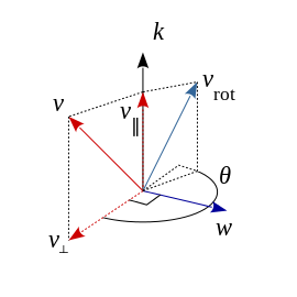
Rodrigues’ rotation formula rotates v by an angle θaround vector k by decomposing it into its components parallel and perpendicular to k, and rotating only the perpendicular component.
Let k be a unit vector defining a rotation axis, and let v be any vector to rotate about k by angle θ (right hand rule, anticlockwise in the figure).
Using the dot and cross products, the vector v can be decomposed into components parallel and perpendicular to the axis k,

- where the component parallel to k is

- called the vector projection of v on k, and the component perpendicular to k is

- called the vector rejection of v from k.
The vector k × v can be viewed as a copy of v⊥ rotated anticlockwise by 90° about k, so their magnitudes are equal but directions are perpendicular. Likewise the vector k × (k × v) a copy of v⊥ rotated anticlockwise through 180° about k, so that k × (k × v) and v⊥ are equal in magnitude but in opposite directions (i.e. they are negatives of each other, hence the minus sign). Expanding the vector triple productestablishes the connection between the parallel and perpendicular components, for reference the formula is a × (b × c) = (a · c)b − (a · b)c given any three vectors a, b, c.
The component parallel to the axis will not change magnitude nor direction under the rotation,

- only the perpendicular component will change direction but retain its magnitude, according to

- and since k and v∥ are parallel, their cross product is zero k × v∥ = 0, so that

- and it follows

- This rotation is correct since the vectors v⊥ and k × v have the same length, and k × v is v⊥ rotated anticlockwise through 90° about k. An appropriate scaling of v⊥ and k × v using the trigonometric functions sine and cosine gives the rotated perpendicular component. The form of the rotated component is similar to the radial vector in 2D planar polar coordinates (r, θ) in the Cartesian basis

- where ex, ey are unit vectors in their indicated directions.
Now the full rotated vector is

- By substituting the definitions of v∥rot and v⊥rot in the equation results in


Vector geometry of Rodrigues’ rotation formula, as well as the decomposition into parallel and perpendicular components.
Matrix notation
Representing v and k × v as column matrices, the cross product can be expressed as a matrix product

- Letting K denote the “cross-product matrix” for the unit vector k,
![\displaystyle \mathbf {K} =\left[{\begin{array}{ccc}0&-k_{z}&k_{y}\\k_{z}&0&-k_{x}\\-k_{y}&k_{x}&0\end{array}}\right]\,,](http://www.freesandal.org/wp-content/ql-cache/quicklatex.com-6dd7dd45d725e0b0b4247e553d45492f_l3.png "Rendered by QuickLaTeX.com")
- the matrix equation is, symbolically,

- for any vector v. (In fact, K is the unique matrix with this property. It has eigenvalues 0 and ±i).
Iterating the cross product on the right is equivalent to multiplying by the cross product matrix on the left, in particular

- Moreover, since k is a unit vector, K has unit 2-norm. The previous rotation formula in matrix language is therefore

- Note the coefficient of the leading term is now 1, in this notation.
Factorizing the v allows the compact expression

- where

is the rotation matrix through an angle θ anticlockwise about the axis k, and I the 3 × 3 identity matrix. This matrix R is an element of the rotation group SO(3) of ℝ3, and K is an element of the Lie algebra so(3) generating that Lie group (note that K is skew-symmetric, which characterizes so(3)). In terms of the matrix exponential,

- To see that the last identity holds, one notes that

- characteristic of a one-parameter subgroup, i.e. exponential, and that the formulas match for infinitesimal θ.
For an alternative derivation based on this exponential relationship, see exponential map from so(3) to SO(3). For the inverse mapping, see log map from SO(3) to so(3).
───
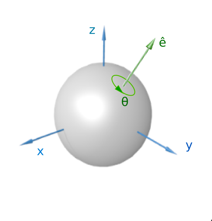
Axis–angle representation
In mathematics, the axis–angle representation of a rotation parameterizes a rotation in a three-dimensional Euclidean space by two quantities: a unit vector e indicating the direction of an axis of rotation, and an angle θ describing the magnitude of the rotation about the axis. Only two numbers, not three, are needed to define the direction of a unit vector e rooted at the origin because the magnitude of e is constrained. For example, the elevation and azimuth angles of esuffice to locate it in any particular Cartesian coordinate frame. The angle θ scalar multiplied by the unit vector e is the axis-angle vector

- The vector itself does not perform rotations, but is used to construct transformations on vectors that correspond to rotations. The rotation occurs in the sense prescribed by the right-hand rule. The rotation axis is sometimes called theEuler axis.
It is one of many rotation formalisms in three dimensions. The axis–angle representation is predicated on Euler’s rotation theorem, which dictates that any rotation or sequence of rotations of a rigid body in a three-dimensional space is equivalent to a pure rotation about a single fixed axis.
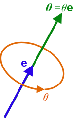
The angle axis vectorθ = θe is a unit vector emultiplied by an angle θ.
Exponential map from so (3) to SO(3)
The exponential map effects a transformation from the axis-angle representation of rotations to rotation matrices,

- Essentially, by using a Taylor expansion one derives a closed-form relation between these two representations. Given a unit vector ω ∈
 (3) = ℝ3 representing the unit rotation axis, and an angle, θ ∈ ℝ, an equivalent rotation matrix R is given as follows, where Kis the cross product matrix of ω, that is, Kv = ω × v for all vectors v ∈ ℝ3,
- Because K is skew-symmetric, and the sum of the squares of its above-diagonal entries is 1, the characteristic polynomial P(t) of K is P(t) = det(K − tI) = −(t3 + t). Since, by the Cayley–Hamilton theorem, P(K) = 0, this implies that

- As a result, K4 = –K2, K5 = K, K6 = K2, K7 = –K.
This cyclic pattern continues indefinitely, and so all higher powers of K can be expressed in terms of K and K2. Thus, from the above equation, it follows that

- that is,

- This is a Lie-algebraic derivation, in contrast to the geometric one in the article Rodrigues’ rotation formula.[1]
Due to the existence of the above-mentioned exponential map, the unit vector ω representing the rotation axis, and the angle θ are sometimes called the exponential coordinates of the rotation matrix R.
因此我們敢篤定的說︰剛體運動可用『定點』之『平移』與相對『定點』的『轉動』來描述!!
Rigid body
In physics, a rigid body is a solid body in which deformation is zero or so small it can be neglected. The distance between any two given points on a rigid body remains constant in time regardless of external forces exerted on it. A rigid body is usually considered as a continuous distribution of mass.
In the study of special relativity, a perfectly rigid body does not exist; and objects can only be assumed to be rigid if they are not moving near the speed of light. In quantum mechanics a rigid body is usually thought of as a collection of point masses. For instance, in quantum mechanics molecules (consisting of the point masses: electrons and nuclei) are often seen as rigid bodies (see classification of molecules as rigid rotors).
Kinematics
Linear and angular position
The position of a rigid body is the position of all the particles of which it is composed. To simplify the description of this position, we exploit the property that the body is rigid, namely that all its particles maintain the same distance relative to each other. If the body is rigid, it is sufficient to describe the position of at least three non-collinear particles. This makes it possible to reconstruct the position of all the other particles, provided that their time-invariant position relative to the three selected particles is known. However, typically a different, mathematically more convenient, but equivalent approach is used. The position of the whole body is represented by:
- the linear position or position of the body, namely the position of one of the particles of the body, specifically chosen as a reference point (typically coinciding with the center of mass or centroid of the body), together with
- the angular position (also known as orientation, or attitude) of the body.
Thus, the position of a rigid body has two components: linear and angular, respectively.[2] The same is true for other kinematic and kinetic quantities describing the motion of a rigid body, such as linear and angular velocity, acceleration, momentum, impulse, andkinetic energy.[3]
The linear position can be represented by a vector with its tail at an arbitrary reference point in space (the origin of a chosen coordinate system) and its tip at an arbitrary point of interest on the rigid body, typically coinciding with its center of mass or centroid. This reference point may define the origin of a coordinate system fixed to the body.
There are several ways to numerically describe the orientation of a rigid body, including a set of three Euler angles, a quaternion, or a direction cosine matrix (also referred to as a rotation matrix). All these methods actually define the orientation of a basis set (orcoordinate system) which has a fixed orientation relative to the body (i.e. rotates together with the body), relative to another basis set (or coordinate system), from which the motion of the rigid body is observed. For instance, a basis set with fixed orientation relative to an airplane can be defined as a set of three orthogonal unit vectors b1, b2, b3, such that b1 is parallel to the chord line of the wing and directed forward, b2 is normal to the plane of symmetry and directed rightward, and b3 is given by the cross product  .
.
In general, when a rigid body moves, both its position and orientation vary with time. In the kinematic sense, these changes are referred to as translation and rotation, respectively. Indeed, the position of a rigid body can be viewed as a hypothetic translation and rotation (roto-translation) of the body starting from a hypothetic reference position (not necessarily coinciding with a position actually taken by the body during its motion).
Linear and angular velocity
Velocity (also called linear velocity) and angular velocity are measured with respect to a frame of reference.
The linear velocity of a rigid body is a vector quantity, equal to the time rate of change of its linear position. Thus, it is the velocity of a reference point fixed to the body. During purely translational motion (motion with no rotation), all points on a rigid body move with the same velocity. However, when motion involves rotation, the instantaneous velocity of any two points on the body will generally not be the same. Two points of a rotating body will have the same instantaneous velocity only if they happen to lie on an axis parallel to the instantaneous axis of rotation.
Angular velocity is a vector quantity that describes the angular speed at which the orientation of the rigid body is changing and the instantaneous axis about which it is rotating (the existence of this instantaneous axis is guaranteed by the Euler’s rotation theorem). All points on a rigid body experience the same angular velocity at all times. During purely rotational motion, all points on the body change position except for those lying on the instantaneous axis of rotation. The relationship between orientation and angular velocity is not directly analogous to the relationship between position and velocity. Angular velocity is not the time rate of change of orientation, because there is no such concept as an orientation vector that can be differentiated to obtain the angular velocity.