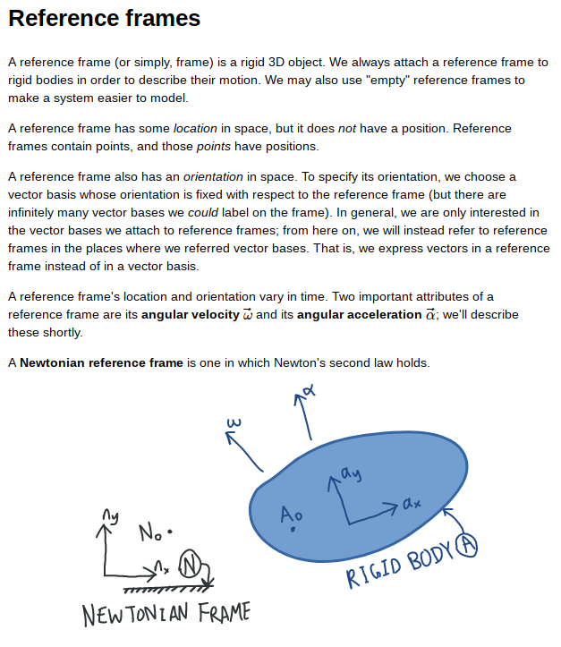
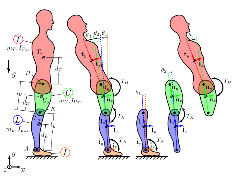
STEM 隨筆︰古典力學︰運動學【二.一】

如果還沒讀過

 Rigid body dynamics is concerned with describing the motion of systems composed of solid bodies; such as vehicles, skeletons, robots [1-4]:

Examples of rigid body systems

This document borrows heavily from [5, 6].


是時候了!

此處擷取其中一段文本,講兩個『參考系定位』之『觀點約定』︰


否則困惑恐生也?

Active and passive transformation

In physics and engineering, an active transformation, or alibi transformation,[1] is a transformation which actually changes the physical position of a point, or rigid body, which can be defined even in the absence of a coordinate system; whereas a passive transformation, or alias transformation,[2] is merely a change in the coordinate system in which the object is described (change of coordinate map, orchange of basis). By default, by transformation, mathematicians usually refer to active transformations, while physicists and engineers could mean either.

Put differently, a passive transformation refers to description of the same object in two different coordinate systems.[3] On the other hand, an active transformation is a transformation of one or more objects with respect to the same coordinate system. For instance, active transformations are useful to describe successive positions of a rigid body. On the other hand, passive transformations may be useful in human motion analysis to observe the motion of the tibia relative to the femur, that is, its motion relative to a (local) coordinate system which moves together with the femur, rather than a (global) coordinate system which is fixed to the floor.[3]

In the active transformation (left), a point moves from position P to P’ by rotating clockwise by an angle θ about the origin of the coordinate system. In the passive transformation (right), point P does not move, while the coordinate system rotates counterclockwise by an angle θ about its origin. The coordinates of P’ in the active case (that is, relative to the original coordinate system) are the same as the coordinates of P relative to the rotated coordinate system.


STEM 隨筆︰古典力學︰運動學【一】

有時文字能使『學問』感覺簡單了!一門『描述運動』之

運動學

運動學(kinematics)是力學的一門分支,專門描述物體的運動,即物體在空間中的位置隨時間的演進而作的改變,完全不考慮作用力質量等等影響運動的因素。運動學與力動學動力學不同。力動學專門研究造成運動或影響運動的各種因素。動力學綜合運動學與力動學在一起,研究力學系統由於力的作用隨著時間演進而造成的運動。[1][2]

在開始研討古典力學時,很自然地應該先思考各種可能的運動樣式,而暫時不將任何造成運動的因素納入考量。這初步探詢的知識就是運動學的學術領域。— 愛德蒙·維特克,質點與剛體分析動力學通論

任何一個物體,像是車子、火箭、星球等等,不論其尺寸大小,假若能夠忽略其內部的相對運動,假若其內部的每一部份都是朝相同的方向、以相同的速度移動,那麼,可以簡易地將此物體視為質點 ,將此物體的質心的位置當作質點的位置。在運動學裏,這種質點運動,不論是直線運動或是曲線運動,都是最基本的研究對象。

假若不能忽略物體內部的相對運動,則當解析其運動時,必須先將物體理想化為剛體,即一群彼此之間距離不變的質點。涉及剛體的問題比較困難。剛體可能會進行平移運動、旋轉運動或兩者的綜合。更困難的案例是多剛體系統的運動。在這系統內,幾個剛體由機械連桿連結在一起。運動學分析某連桿裝置的可能運動範圍,或反過來,設計滿足預定運動範圍的連桿裝置。起重機或引擎活塞系統都是簡單的運動系統。起重機是一種開運動鏈。活塞系統是四連桿組的一部分。

掛在重力式摩天輪邊緣的乘客座艙在做平移運動

……

Kinematics

Kinematics is a branch of classical mechanics that describes the motion of points, bodies (objects), and systems of bodies (groups of objects) without considering the mass of each or the forces that caused the motion.[1][2][3] Kinematics, as a field of study, is often referred to as the “geometry of motion” and is occasionally seen as a branch of mathematics.[4][5][6] A kinematics problem begins by describing the geometry of the system and declaring the initial conditions of any known values of position, velocity and/or acceleration of points within the system. Then, using arguments from geometry, the position, velocity and acceleration of any unknown parts of the system can be determined. The study of how forces act on masses falls within kinetics. For further details, see analytical dynamics.

Kinematics is used in astrophysics to describe the motion of celestial bodies and collections of such bodies. In mechanical engineering, robotics, and biomechanics[7] kinematics is used to describe the motion of systems composed of joined parts (multi-link systems) such as an engine, a robotic arm or the human skeleton.

Geometric transformations, also called rigid transformations, are used to describe the movement of components in a mechanical system, simplifying the derivation of the equations of motion. They are also central todynamic analysis.

Kinematic analysis is the process of measuring the kinematic quantities used to describe motion. In engineering, for instance, kinematic analysis may be used to find the range of movement for a given mechanism, and working in reverse, using kinematic synthesis to design a mechanism for a desired range of motion.[8] In addition, kinematics applies algebraic geometry to the study of the mechanical advantage of a mechanical system or mechanism.

───


能有多困難的呢?如果聽聽

AUTHOR
Kane, Thomas R.; Levinson, David A.
ABSTRACT
This textbook is intended to provide a basis for instruction in dynamics. Its purpose is not only to equip students with the skills they need to deal effectively with present-day dynamics problems, but also to bring them into position to interact smoothly with those trained more conventionally.


書中,第二章起頭處作者之說法︰


怕是不通『運動學』,恐難掌握『動力學』哩!!

因此所以借

/pydy-tutorial-human-standing

PyDy tutorial materials for MASB 2014, PYCON 2014, and SciPy 2014/2015. http://pydy.org

Example Problem

The tutorial will go through the PyDy workflow in small steps. At the end the students should have a working 3-link 2D inverted pendulum model of a human that can be used for balancing studies. The free body diagram of the model is shown below:

notebooks/figures/human_balance_diagram.png

……

Notebooks

These are the notebooks for the tutorial.


串講補充耶??

 The first step, and notably the most difficult, is to define the kinematic relationships (i.e. motion) among rigid bodies in the system. Here will we make use of ReferenceFrameobjects to describe the four frames in the problem, set their orientations, and then construct vectors in the frames that position various important Points. Finally, we will specify the linear and angular velocities of the frames and points using generalized speeds.


也許世間物只要『部件很多』自然『複雜』的乎?!


STEM 隨筆︰古典力學︰慣性系【三】

藉著認識『慣性力』,又稱『假想力』︰

Fictitious force

A fictitious force (also called a pseudo force,[1] d’Alembert force,[2][3] or inertial force[4][5]) is an apparent force that acts on all masses whose motion is described using a non-inertial frame of reference, such as a rotating reference frame. Examples are the forces that act on passengers in an accelerating or braking automobile, and the force that pushes objects toward the rim of a centrifuge.

The fictitious force F is due to an object’s inertia when the reference frame does not move inertially, and thus begins to accelerate relative to the free object. The fictitious force thus does not arise from any physical interaction between two objects (that is, it is not a “contact force”), but rather from the acceleration a of the non-inertial reference frame itself, which from the viewpoint of the frame now appears to be an acceleration of the object instead, requiring a “force” to make this happen. As stated by Iro:[6][7]

Such an additional force due to nonuniform relative motion of two reference frames is called a pseudo-force.

— H. Iro in A Modern Approach to Classical Mechanics p. 180

Assuming Newton’s second law in the form F = ma, fictitious forces are always proportional to the mass m.

The fictitious force on an object arises as an imaginary influence, when the frame of reference used to describe the object’s motion is accelerating compared to a non-accelerating frame. The fictitious force “explains,” using Newton’s mechanics, why an object does not follow Newton’s laws and “float freely” as if weightless. As a frame can accelerate in any arbitrary way, so can fictitious forces be as arbitrary (but only in direct response to the acceleration of the frame). However, four fictitious forces are defined for frames accelerated in commonly occurring ways: one caused by any relative acceleration of the origin in a straight line (rectilinear acceleration);[8]two involving rotation: centrifugal force and Coriolis force; and a fourth, called the Euler force, caused by a variable rate of rotation, should that occur.

Gravitational force would also be a fictitious force based upon a field model in which particles distort spacetime due to their mass, such as General Relativity.


知道如何數學推導︰

Mathematical derivation of fictitious forces

General derivation

Many problems require use of noninertial reference frames, for example, those involving satellites[21][22] and particle accelerators.[23] Figure 2 shows a particle with mass m and position vector xA(t) in a particular inertial frame A. Consider a non-inertial frame B whose origin relative to the inertial one is given by XAB(t). Let the position of the particle in frame B be xB(t). What is the force on the particle as expressed in the coordinate system of frame B? [24][25]

To answer this question, let the coordinate axis in B be represented by unit vectors uj with j any of { 1, 2, 3 } for the three coordinate axes. Then

\displaystyle \mathbf {x} _{\mathrm {B} }=\sum _{j=1}^{3}x_{j}\mathbf {u} _{j}\ .

The interpretation of this equation is that xB is the vector displacement of the particle as expressed in terms of the coordinates in frame B at time t. From frame A the particle is located at:
\displaystyle \mathbf {x} _{\mathrm {A} }=\mathbf {X} _{\mathrm {AB} }+\sum _{j=1}^{3}x_{j}\mathbf {u} _{j}\ .
As an aside, the unit vectors { uj } cannot change magnitude, so derivatives of these vectors express only rotation of the coordinate system B. On the other hand, vector XAB simply locates the origin of frame B relative to frame A, and so cannot include rotation of frame B.

Taking a time derivative, the velocity of the particle is:

\displaystyle {\frac {d\mathbf {x} _{\mathrm {A} }}{dt}}={\frac {d\mathbf {X} _{\mathrm {AB} }}{dt}}+\sum _{j=1}^{3}{\frac {dx_{j}}{dt}}\mathbf {u} _{j}+\sum _{j=1}^{3}x_{j}{\frac {d\mathbf {u} _{j}}{dt}}\ .

The second term summation is the velocity of the particle, say vB as measured in frame B. That is:
\displaystyle {\frac {d\mathbf {x} _{\mathrm {A} }}{dt}}=\mathbf {v} _{\mathrm {AB} }+\mathbf {v} _{\mathrm {B} }+\sum _{j=1}^{3}x_{j}{\frac {d\mathbf {u} _{j}}{dt}}.
The interpretation of this equation is that the velocity of the particle seen by observers in frame A consists of what observers in frame B call the velocity, namely vB, plus two extra terms related to the rate of change of the frame-B coordinate axes. One of these is simply the velocity of the moving origin vAB. The other is a contribution to velocity due to the fact that different locations in the non-inertial frame have different apparent velocities due to rotation of the frame; a point seen from a rotating frame has a rotational component of velocity that is greater the further the point is from the origin.

To find the acceleration, another time differentiation provides:

\displaystyle {\frac {d^{2}\mathbf {x} _{\mathrm {A} }}{dt^{2}}}=\mathbf {a} _{\mathrm {AB} }+{\frac {d\mathbf {v} _{\mathrm {B} }}{dt}}+\sum _{j=1}^{3}{\frac {dx_{j}}{dt}}{\frac {d\mathbf {u} _{j}}{dt}}+\sum _{j=1}^{3}x_{j}{\frac {d^{2}\mathbf {u} _{j}}{dt^{2}}}.

Using the same formula already used for the time derivative of xB, the velocity derivative on the right is:
\displaystyle {\frac {d\mathbf {v} _{\mathrm {B} }}{dt}}=\sum _{j=1}^{3}{\frac {dv_{j}}{dt}}\mathbf {u} _{j}+\sum _{j=1}^{3}v_{j}{\frac {d\mathbf {u} _{j}}{dt}}=\mathbf {a} _{\mathrm {B} }+\sum _{j=1}^{3}v_{j}{\frac {d\mathbf {u} _{j}}{dt}}.
Consequently,
\displaystyle {\frac {d^{2}\mathbf {x} _{\mathrm {A} }}{dt^{2}}}=\mathbf {a} _{\mathrm {AB} }+\mathbf {a} _{\mathrm {B} }+2\ \sum _{j=1}^{3}v_{j}{\frac {d\mathbf {u} _{j}}{dt}}+\sum _{j=1}^{3}x_{j}{\frac {d^{2}\mathbf {u} _{j}}{dt^{2}}}.
     
 
(1)

The interpretation of this equation is as follows: the acceleration of the particle in frame A consists of what observers in frame B call the particle acceleration aB, but in addition there are three acceleration terms related to the movement of the frame-B coordinate axes: one term related to the acceleration of the origin of frame B, namely aAB, and two terms related to rotation of frame B. Consequently, observers in B will see the particle motion as possessing “extra” acceleration, which they will attribute to “forces” acting on the particle, but which observers in A say are “fictitious” forces arising simply because observers in B do not recognize the non-inertial nature of frame B.

The factor of two in the Coriolis force arises from two equal contributions: (i) the apparent change of an inertially constant velocity with time because rotation makes the direction of the velocity seem to change (a dvB/dt term) and (ii) an apparent change in the velocity of an object when its position changes, putting it nearer to or further from the axis of rotation (the change in \displaystyle \sum x_{j}\,d\mathbf {u} _{j}/dt  due to change in x j ).

To put matters in terms of forces, the accelerations are multiplied by the particle mass:

\displaystyle \mathbf {F} _{\mathrm {A} }=\mathbf {F} _{\mathrm {B} }+m\mathbf {a} _{\mathrm {AB} }+2m\sum _{j=1}^{3}v_{j}{\frac {d\mathbf {u} _{j}}{dt}}+m\sum _{j=1}^{3}x_{j}{\frac {d^{2}\mathbf {u} _{j}}{dt^{2}}}\ .

The force observed in frame B, FB = maB is related to the actual force on the particle, FA, by
\displaystyle \mathbf {F} _{\mathrm {B} }=\mathbf {F} _{\mathrm {A} }+\mathbf {F} _{\mathrm {fictitious} },
where:
\displaystyle \mathbf {F} _{\mathrm {fictitious} }=-m\mathbf {a} _{\mathrm {AB} }-2m\sum _{j=1}^{3}v_{j}{\frac {d\mathbf {u} _{j}}{dt}}-m\sum _{j=1}^{3}x_{j}{\frac {d^{2}\mathbf {u} _{j}}{dt^{2}}}\ .
Thus, we can solve problems in frame B by assuming that Newton’s second law holds (with respect to quantities in that frame) and treating Ffictitious as an additional force.[12][26][27]

Below are a number of examples applying this result for fictitious forces. More examples can be found in the article on centrifugal force.

Rotating coordinate systems

A common situation in which noninertial reference frames are useful is when the reference frame is rotating. Because such rotational motion is non-inertial, due to the acceleration present in any rotational motion, a fictitious force can always be invoked by using a rotational frame of reference. Despite this complication, the use of fictitious forces often simplifies the calculations involved.

To derive expressions for the fictitious forces, derivatives are needed for the apparent time rate of change of vectors that take into account time-variation of the coordinate axes. If the rotation of frame ‘B’ is represented by a vector Ω pointed along the axis of rotation with orientation given by the right-hand rule, and with magnitude given by

\displaystyle |{\boldsymbol {\Omega }}|={\frac {d\theta }{dt}}=\omega (t),

then the time derivative of any of the three unit vectors describing frame B is[26][28]
\displaystyle {\frac {d\mathbf {u} _{j}(t)}{dt}}={\boldsymbol {\Omega }}\times \mathbf {u} _{j}(t),
and
\displaystyle {\frac {d^{2}\mathbf {u} _{j}(t)}{dt^{2}}}={\frac {d{\boldsymbol {\Omega }}}{dt}}\times \mathbf {u} _{j}+{\boldsymbol {\Omega }}\times {\frac {d\mathbf {u} _{j}(t)}{dt}}={\frac {d{\boldsymbol {\Omega }}}{dt}}\times \mathbf {u} _{j}+{\boldsymbol {\Omega }}\times \left[{\boldsymbol {\Omega }}\times \mathbf {u} _{j}(t)\right],
as is verified using the properties of the vector cross product. These derivative formulas now are applied to the relationship between acceleration in an inertial frame, and that in a coordinate frame rotating with time-varying angular velocity ω(t). From the previous section, where subscript A refers to the inertial frame and B to the rotating frame, setting aAB = 0 to remove any translational acceleration, and focusing on only rotational properties (see Eq. 1):
\displaystyle {\frac {d^{2}\mathbf {x} _{\mathrm {A} }}{dt^{2}}}=\mathbf {a} _{\mathrm {B} }+2\sum _{j=1}^{3}v_{j}\ {\frac {d\mathbf {u} _{j}}{dt}}+\sum _{j=1}^{3}x_{j}{\frac {d^{2}\mathbf {u} _{j}}{dt^{2}}},
\displaystyle \mathbf {a} _{\mathrm {A} }=\mathbf {a} _{\mathrm {B} }+\ 2\sum _{j=1}^{3}v_{j}{\boldsymbol {\Omega }}\times \mathbf {u} _{j}(t)+\sum _{j=1}^{3}x_{j}{\frac {d{\boldsymbol {\Omega }}}{dt}}\times \mathbf {u} _{j}\ +\sum _{j=1}^{3}x_{j}{\boldsymbol {\Omega }}\times \left[{\boldsymbol {\Omega }}\times \mathbf {u} _{j}(t)\right]
\displaystyle =\mathbf {a} _{\mathrm {B} }+2{\boldsymbol {\Omega }}\times \sum _{j=1}^{3}v_{j}\mathbf {u} _{j}(t)+{\frac {d{\boldsymbol {\Omega }}}{dt}}\times \sum _{j=1}^{3}x_{j}\mathbf {u} _{j}+{\boldsymbol {\Omega }}\times \left[{\boldsymbol {\Omega }}\times \sum _{j=1}^{3}x_{j}\mathbf {u} _{j}(t)\right].

Collecting terms, the result is the so-called acceleration transformation formula:[29]
\displaystyle \mathbf {a} _{\mathrm {A} }=\mathbf {a} _{\mathrm {B} }+2{\boldsymbol {\Omega }}\times \mathbf {v} _{\mathrm {B} }+{\frac {d{\boldsymbol {\Omega }}}{dt}}\times \mathbf {x} _{\mathrm {B} }+{\boldsymbol {\Omega }}\times \left({\boldsymbol {\Omega }}\times \mathbf {x} _{\mathrm {B} }\right)\ .
The physical acceleration aA due to what observers in the inertial frame A call real external forces on the object is, therefore, not simply the acceleration aB seen by observers in the rotational frame B, but has several additional geometric acceleration terms associated with the rotation of B. As seen in the rotational frame, the acceleration aB of the particle is given by rearrangement of the above equation as:
\displaystyle \mathbf {a} _{\mathrm {B} }=\mathbf {a} _{\mathrm {A} }-2{\boldsymbol {\Omega }}\times \mathbf {v} _{\mathrm {B} }-{\boldsymbol {\Omega }}\times ({\boldsymbol {\Omega }}\times \mathbf {x} _{\mathrm {B} })-{\frac {d{\boldsymbol {\Omega }}}{dt}}\times \mathbf {x} _{\mathrm {B} }.
The net force upon the object according to observers in the rotating frame is FB = maB. If their observations are to result in the correct force on the object when using Newton’s laws, they must consider that the additional force Ffict is present, so the end result is FB =FA + Ffict. Thus, the fictitious force used by observers in B to get the correct behavior of the object from Newton’s laws equals:
\displaystyle \mathbf {F} _{\mathrm {fict} }=-2m{\boldsymbol {\Omega }}\times \mathbf {v} _{\mathrm {B} }-m{\boldsymbol {\Omega }}\times ({\boldsymbol {\Omega }}\times \mathbf {x} _{\mathrm {B} })-m{\frac {d{\boldsymbol {\Omega }}}{dt}}\times \mathbf {x} _{\mathrm {B} }.
Here, the first term is the Coriolis force,[30] the second term is the centrifugal force,[31] and the third term is the Euler force.[32][33]


自能深入了解 Sympy Kinematics 所說 v1pt 、 v2pt 理論︰

v1pt_theory(otherpoint, outframe, interframe)

Sets the velocity of this point with the 1-point theory.

The 1-point theory for point velocity looks like this:

^N v^P = ^B v^P + ^N v^O + ^N omega^B x r^OP

where O is a point fixed in B, P is a point moving in B, and B is rotating in frame N.

PARAMETERS :

otherpoint : Point

The first point of the 2-point theory (O)

outframe : ReferenceFrame

The frame we want this point’s velocity defined in (N)

interframe : ReferenceFrame

The intermediate frame in this calculation (B)

Examples

>>> from sympy.physics.mechanics import Point, ReferenceFrame, dynamicsymbols
>>> q = dynamicsymbols('q')
>>> q2 = dynamicsymbols('q2')
>>> qd = dynamicsymbols('q', 1)
>>> q2d = dynamicsymbols('q2', 1)
>>> N = ReferenceFrame('N')
>>> B = ReferenceFrame('B')
>>> B.set_ang_vel(N, 5 * B.y)
>>> O = Point('O')
>>> P = O.locatenew('P', q * B.x)
>>> P.set_vel(B, qd * B.x + q2d * B.y)
>>> O.set_vel(N, 0)
>>> P.v1pt_theory(O, N, B)
q'*B.x + q2'*B.y - 5*q*B.z

v2pt_theory(otherpoint, outframe, fixedframe)

Sets the velocity of this point with the 2-point theory.

The 2-point theory for point velocity looks like this:

^N v^P = ^N v^O + ^N omega^B x r^OP

where O and P are both points fixed in frame B, which is rotating in frame N.

PARAMETERS :

otherpoint : Point

The first point of the 2-point theory (O)

outframe : ReferenceFrame

The frame we want this point’s velocity defined in (N)

fixedframe : ReferenceFrame

The frame in which both points are fixed (B)

Examples

>>> from sympy.physics.mechanics import Point, ReferenceFrame, dynamicsymbols
>>> q = dynamicsymbols('q')
>>> qd = dynamicsymbols('q', 1)
>>> N = ReferenceFrame('N')
>>> B = N.orientnew('B', 'Axis', [q, N.z])
>>> O = Point('O')
>>> P = O.locatenew('P', 10 * B.x)
>>> O.set_vel(N, 5 * N.x)
>>> P.v2pt_theory(O, N, B)
5*N.x + 10*q'*B.y


STEM 隨筆︰古典力學︰慣性系【二】

什麼是

慣性

物理學裡,慣性英語:inertia)是物體抵抗其運動狀態被改變的性質。物體的慣性可以用其質量來衡量,質量越大,慣性也越大 。艾薩克·牛頓在鉅著《自然哲學的數學原理》裡定義慣性為:[1]

慣性,或物質固有的力,是一種抵抗的現象,它存在於每一物體當中 ,大小與該物體相當,並盡量使其保持現有的狀態,不論是靜止狀態,或是勻速直線運動狀態。

更具體而言,牛頓第一定律表明,存在某些參考系,在其中,不受外力的物體都保持靜止或勻速直線運動。也就是說,從某些參考系觀察,假若施加於物體的淨外力為零,則物體運動速度的大小與方向恆定。慣性定義為,牛頓第一定律中的物體具有保持原來運動狀態的性質。滿足牛頓第一定律的參考系,稱為慣性參考系。稍後會有關於慣性參考系的更詳細論述。

慣性原理古典力學的基礎原理。很多學者認為慣性原理就是牛頓第一定律。遵守這原理,物體會持續地以現有速度移動,除非有外力迫使改變其速度。

地球表面,慣性時常會被摩擦力空氣阻力等等效應掩蔽,從而促使物體的移動速度變得越來越慢(通常最後會變成靜止狀態)。這現象誤導了許多古代學者,例如,亞里斯多德認為,在宇宙裡,所有物體都有其「自然位置」──處於完美狀態的位置,物體會固定不動於其自然位置,只有當外力施加時,物體才會移動。[2]


呢?且來段古今走馬看花︰

古典慣性

尼古拉·哥白尼於1543年發表著作《天體運行論》,主張地球(與處於其表面的所有物體)從未停止不動,而是持續地繞著太陽做公轉。面對這嶄新的理論,亞里斯多德式的地心說──地球是宇宙的中心,因此絕對地固定不動──顯得漏洞百出、難以招架。[17]在發表著作之前,哥白尼為了證實自己的理論,早已於1530年就完成了觀測行星軌道運動的實驗。[18]

德國天文學者克卜勒,在從1618年至1621年分三階段發表的著作《哥白尼天文學概要》裡,最先提出術語「慣性」,拉丁語為「懶惰」的意思,與當今的詮釋不太一樣。克卜勒以對於運動變化的抗拒來定義慣性,這仍舊是根據亞里斯多德的靜止狀態為自然狀態的前提。一直要等到後來伽利略的研究與牛頓將靜止與運動統一於同一原理,術語慣性才能應用於當今其所賦有的概念。


伽利略用來檢驗慣性定律的斜面實驗。

伽利略·伽利萊主張,施加外力改變的是物體的速度而不是位置;維持物體速度不變,不需要任何外力。為了證實他的主張,伽利略做了一個思想實驗。如右圖所示,讓靜止的小球從點A滾下斜面AB,滾到最底端後,小球又會滾上斜面BC,假設兩塊斜面都非常的平滑 、摩擦係數極小,而且空氣阻力微弱,以至於可以忽略不計,則小球會滾到與點A同高度的點C;假設斜面是BD、BE或BF,小球也同樣地會滾到與點A同高度的位置。只不過斜面越長 ,往上滾的時候 ,單位時間內速度的減少量會變得越小。假設斜面逐漸延長,最後變成水平面BH,則基於「連續性原則」該小球「本應當」回到與點A同高度的位置,然而由於事實上BH是水平的,小球永遠不可能滾到先前的高度,而速度的減少量將變成0,因此小球會不停地呈勻速直線運動。伽利略總結,假若不碰到任何阻礙,那麼運動中的物體會持續地做勻速直線運動。他將此稱為慣性定律[19][20] 

這理論剛被提出時並不被其他學者接受,因為當時大多數學者不了解摩擦力與空氣阻力的本質,不過伽利略的實驗以可靠的事實為基礎,經過抽象思維,抓住主要因素,忽略次要因素,更深刻地反應了自然規律。

值得注意的是,後來,伽利略從慣性定律推論,假若沒有任何外在參考比較,則絕對無法分辨物體是靜止不動還是移動。這觀察後來成為愛因斯坦發展狹義相對論的基礎。 [21]

好幾位其他自然哲學家與科學家似乎分別獨立地想出了慣性定律[註 1]。第17世紀哲學家勒內·笛卡兒也曾經提出慣性定律,雖然他沒有做出任何實驗來證實這定律的正確性。

牛頓第一定律其實正是伽利略所提出的慣性定律的再次陳述[22]──不施加外力,則沒有加速度,因此物體會維持速度不變。牛頓將這定律的最初提出歸功於伽利略。牛頓第一定律為[23]

物體會保持其靜止或勻速直線運動狀態,除非有外力迫使改變其狀態。

寫出牛頓第一定律後,牛頓開始描述他所觀察到的各種物體的自然運動。像飛箭、飛石一類的拋體,假若不被空氣的阻力抗拒,不被重力吸引墜落,它們會速度不變地持續運動。像陀螺一類的旋轉體 ,假若不受到地面的摩擦力損耗,它們會永久不息地旋轉。像行星彗星一類的星體,在阻力較小的太空中移動,會更長久地維持它們的運動軌道。在這裡,牛頓並沒有提到牛頓第一定律與慣性參考系之間的關係,他所專注的問題是,為什麼在一般觀察中,運動中的物體最終會停止運動?他認為原因是有空氣阻力、地面摩擦力等等作用於物體。假若這些力不存在,則運動中的物體會永遠不停的做勻速運動。這想法是很重要的突破,需要極為仔細的洞察力與豐富的想像力才能達成。

相對論

阿爾伯特·愛因斯坦於1905年在論文《論動體的電動力學》裡提出的狹義相對論,是建立於伽利略與牛頓研究出來的慣性與慣性參考系。儘管這劃時代的理論實際地改變了許多牛頓概念,像質量、能量、距離,那時後,愛因斯坦的慣性概念與牛頓的原本概念絲毫沒有任何差異。實際而言,整個理論是建立於牛頓的慣性定義。但這也使得狹義相對論的相對性原理只能應用於慣性參考系。在這種參考系裡,不受外力的物體,必定保持其靜止或勻速直線運動狀態。為了處理這局限,愛因斯坦於1916年發表論文《廣義相對論的基礎 》提出廣義相對論。這理論能夠應用於非慣性參考系。但是,為了達到這目的,愛因斯坦發覺,他必需使用到彎曲時空的新概念,而不是傳統的牛頓力的概念,來重新定義幾個基礎概念(例如重力) 。

因為這重新定義,愛因斯坦還以測地誤差重新定義了慣性的概念,這又引起一些微妙但重要的結果。根據廣義相對論,當處理大尺寸問題時,不能使用與倚賴傳統牛頓慣性。幸運地,對於足夠小的時空區域,狹義相對論仍舊適用,慣性的內涵與工作仍舊與古典模型相同。

狹義相對論的另一個深奧的結果是,能量與質量不是互不相干的物理屬性,而是可互相轉換的。這嶄新關係也給予慣性概念新的內涵 。狹義相對論的邏輯結果是,假若質量遵守慣性原理,則能量必也遵守慣性原理。對於很多狀況,這理論大大地拓寬了慣性的定義,能夠應用於物質與能量。


彷彿中有所感吧!

再瀏覽多種多方

詮釋

質量與慣性

慣性的定性定義為物體抵抗動量改變的性質。將這定義加以定量延伸為物體抵抗動量改變的度量,就可以用來做數學計算。這度量稱為慣性質量,簡稱為質量。所以,質量表示物質的數量,同時,質量也是物體慣性的度量。

動量方程式表達物體的動量 \vec{p} 與質量 m 、速度 \vec{v} 之間的關係:

\vec{p} = m \cdot \vec{v} 。

但是,牛頓第二定律方程式也可以表達物體的作用力 \vec{F} 與質量(慣性質量)m 、加速度 \vec{a} 之間的關係:

\vec{F} = m \cdot \vec{a} 。

按照這個方程式,給定作用力,則質量越大,加速度越小。由動量方程式與牛頓方程式給出的質量相同。因為,假若質量與時間、速度無關,則牛頓方程式可以從動量方程式推導出來。

這樣,質量是物體慣性的度量,即物體抵抗被加速的度量。物體慣性這詞語的含意,已從原本含意──維持動量的傾向,改變為物體抵抗動量改變的度量。

重力質量與慣性質量

重力質量與慣性質量之間的唯一差別是測量方法。

將未知質量的物體與已知質量的物體分別感受到的重力做測量比較,就可以得到未知物體的重力質量。通常,可以使用天平來做測量。這方法的優點是,不論在甚麼地方,在甚麼星球,都可以用天平來做測量,因為對於任意物體,重力場都一樣。只要重力場不改變,天平會測量出可信的重力質量。但是,在超質量星體附近,例如,黑洞中子星,就不能採用這種方法,因為在這區域裡,重力場的梯度太過陡峭,在天平的左右兩個托盤位置的重力場差異量太大,超過允許誤差範圍。在失重環境,也不能採用這種方法,因為天平不能做任何比較。

施加已知作用力於未知質量的物體,測量產生的加速度,然後應用牛頓第二定律方程式,就可以得到慣性質量,其誤差只限制於測量的準確度。當處於自由落體狀況時,使用這方法,坐在一種特別座椅,稱為物體質量測表,就可以測量出失重航天員的慣性質量。

值得注意的是,實驗者尚未找出,重力質量與慣性質量,兩者之間有甚麼差異。實驗者已完成許多實驗,檢驗兩者的實驗數值,但是差異都在實驗誤差邊限之內。愛因斯坦在創建廣義相對論時,從重力質量與慣性質量相等的事實,得到很大的啟示。他假設重力質量與慣性質量相同,重力所產生的加速度是時空連續統內的斜度所造成的結果,就好像圓球以螺旋線樣式滾下一個倒圓錐

慣性參考系

當描述物體運動時,只有相對於特定的參考系,才能確實顯示出其物理行為。假若選擇了不適當的參考系,則相關的運動定律可能會比較複雜,在慣性參考系中,力學定律表現出的形式最為簡單。[24]從慣性參考系觀察,任何呈勻速直線運動的參考系,也都是慣性參考系,否則是「非慣性參考系」。換句話說,牛頓定律滿足伽利略不變性,即在所有慣性參考系裡,牛頓定律都保持不變[25]

選擇以固定星體來近似慣性參考系,這方法的誤差相當微小。例如,地球繞著太陽的公轉所產生的離心力,比太陽繞著銀河系中心的公轉所產生的離心力,要大三千萬倍。所以,在研究太陽系星體的運動時,太陽是一個很好的慣性參考系。[26]地球也可以視為慣性參考系。由於地球自轉而產生的加速度在地球表面為0.034m· s-2重力加速度大約為自轉加速度的288倍。由於地球繞著太陽公轉而產生的加速度為0.006m· s-2,更為微小。所以,可以忽略地球的自轉和公轉加速度。[27]

假設處於地球參考系的觀察者A,觀察到一輛火車呈勻速直線運動,則附著於此火車的參考系(火車參考系)也是慣性參考系。現在,在火車車廂內,有一個圓球從高處掉落下來,處於火車參考系的觀察者B,所觀察到的圓球軌跡,就如同當這火車固定不動時,這圓球會垂直掉落下來一樣。從地球參考系觀察,在掉落之前,圓球與火車的移動速度與方向相同,圓球的慣性保證,朝著火車移動方向,圓球與火車的移動速度相等。注意到在這裡,是慣性而不是質量給出這保證。

每一個慣性參考系裡的觀察者,都會觀察到所有物理行為都遵守同樣的物理定律。從一個慣性參考系,可以簡單又直覺明顯地變換(伽利略變換)到另外一個慣性參考系。這樣,處於地球參考系的觀測者A能夠推論,火車參考系的觀察者B會觀察到,在火車車廂內掉落的圓球,會垂直掉落下來。

對於非慣性參考系而言,由於參考系的加速度不等於零,物體會感受到虛設力。假設火車正在加速度中,則火車參考系的觀察者B會觀察到,圓球不會垂直地掉落,而會偏改方向,這是因為朝著火車移動方向,圓球與火車的移動速度不相等。

再舉一個例子,假設將地球自轉納入考量,地球每24小時會自轉一週,旋轉的地球參考系是非慣性參考系。從北極發設一枚飛彈,對準南方位於赤道的某點P,則從地球參考系觀察,由於感受到科里奧利力,這枚飛彈會偏離點P。但是,從太陽參考系觀察,由於地球的自轉,點P位置有所改變,所以沒有準確抵達點P。

慣性的起源

牛頓特別定義絕對空間為不依賴於外界任何事物而獨自存在的參考系,在絕對時空中,不受力的物體具有保持原來運動狀態的性質,這性質稱為「慣性」。牛頓認為慣性是物體的內秉性質。

恩斯特·馬赫認為,絕對空間的概念太過玄秘,絕對空間不是可以實際觀察測得。假若將所有遙遠星體的運動平均,得到的參考系應該是靜止的,可以替代絕對空間。因此,物體的慣性與遙遠的星體有關,物體的慣性起源於其與整個宇宙的物質之間的交互作用,也就是說,「遠域的物質決定了本域的慣性」。但是,遠在宇宙的那一端,相距109光年宇宙半徑的星球,怎麼能夠影響本域的慣性?儘管馬赫的批評很有道理,牛頓力學的準確度是有眼共睹的事實。究竟是甚麼原因造成了遠域的物質似乎與本域的慣性沒甚麼牽連的表象?

愛因斯坦在研究廣義相對論時,深深地被馬赫的理論吸引與啟發,愛因斯坦稱這想法為馬赫原理。愛因斯坦表明,重力是遙遠物質影響本域慣性的機制,而這耦合發生於彎曲時空,可以用幾何動力學的初值方程式計算求得。根據愛因斯坦的理論,只要知道宇宙的整個質量-能量分布與流動,就可以計算出,在任意位置與時間,物體的慣性。這具體地給出了馬赫定理的操作機制。[28]

假設一個旋轉圓球殼的質量等於地球質量、半徑等於地球半徑、旋轉角速度等於地球自轉角速度,在圓心位置有一個傅科擺,則這旋轉圓球殼對於傅科擺產生的參考系拖曳現象,與整個宇宙對於傅科擺產生的現象,兩者之間的比率大約為5×10-14。因此,可以結論地球對於傅科擺的影響相當微小。假若地球質量加大0.2×10¹⁴倍,則旋轉圓球殼對於傅科擺產生的參考系拖曳現象相當於宇宙對於傅科擺產生的現象。[28]

轉動慣量

工業飛輪具有很大的轉動慣量,可以用來抵抗轉速的改變。當動力源對旋轉軸作用有一個變動的力矩時(例如往複式發動機),或是應用在間歇性負載時(例如活塞沖床),飛輪可以減小轉速的波動,使旋轉運動更加平順。

轉動慣量是慣性的另外一種形式,指的是剛體在旋轉時維持其勻速旋轉運動的傾向。除非有外力矩施加,剛體的角動量不會改變。這理論稱為角動量守恆定律。由於陀螺儀的轉動慣量,它可以抵抗任何對於旋轉軸方向的改變。


,朦朧裡有所覺乎??

這樣『學』、『思』者,大概不會問『宇宙大霹靂』前、中、後『動量變化』哩★

今日談『思』與『學』,幸有其人可效法也!!

☆ 緬懷

史蒂芬·霍金

史蒂芬·霍金攝於美國國家航空暨太空總署

史蒂芬·威廉·霍金CHCBEFRSFRSA英語:Stephen William Hawking,1942年1月8日-2018年3月14日[2]),英國物理學家宇宙學家,及書籍作者,生前任職劍橋大學理論宇宙學中心研究主任[3][4]。他在科學上有許多貢獻,包括與羅傑·潘洛斯共同合作提出在廣義相對論框架內的潘洛斯–霍金奇性定理,以及他對關於黑洞會發放輻射的理論性預測(現稱為霍金輻射)。霍金是第一個提出由廣義相對論和量子力學聯合解釋的宇宙論理論之人。他是量子力學的多世界詮釋的積極支持者[5][6]

霍金是皇家文藝學會獎(FRSA)的得獎者,並成為宗座科學院的終身會員,並曾經獲得總統自由勳章,是美國所頒發最高榮譽的平民獎。2002年,霍金在BBC的「最偉大的100名英國人」民意調查中位列第25位。從1979年至2009年,霍金是劍橋大學盧卡斯數學教授。霍金撰寫了多本闡述自己理論與一般宇宙論的科普著作,並廣受大眾歡迎。他的著作《時間簡史:從大爆炸到黑洞》曾經破紀錄地榮登英國《星期日泰晤士報》的暢銷書排行榜共計237周[7]:1

霍金患有一種罕見的早發性緩慢進展的運動神經元疾病(也稱為肌萎縮性脊髓側索硬化症或稱為ALS或盧·賈里格症),病情會隨著年月逐漸惡化至嚴重[8][9]。他晚年已是全身癱瘓,無法發聲,必須依賴語音產生裝置來與其他人溝通。最初裝置透過手持開關來使用,最終需要透過使用單邊臉頰肌肉。

2018年3月14日,霍金的家人發表聲明表示霍金去世,終年76歲 。[10][11]


終究 STEM 一直是『實踐者』之園地!!??