W!o+ 的《小伶鼬工坊演義》︰神經網絡【學而堯曰】一

Michael Nielsen 先生之第三章讀來十分有趣,首起

【學習指南】

《論語》‧《學而
子曰:「學而時習之,不亦說乎?有朋自遠方來,不亦樂乎?人不知而不慍,不亦君子乎?

孔子說:「經常學習,不也喜悅嗎?遠方來了朋友,不也快樂嗎?得不到理解而不怨恨,不也是君子嗎?」


When a golf player is first learning to play golf, they usually spend most of their time developing a basic swing. Only gradually do they develop other shots, learning to chip, draw and fade the ball, building on and modifying their basic swing. In a similar way, up to now we’ve focused on understanding the backpropagation algorithm. It’s our “basic swing”, the foundation for learning in most work on neural networks. In this chapter I explain a suite of techniques which can be used to improve on our vanilla implementation of backpropagation, and so improve the way our networks learn.

The techniques we’ll develop in this chapter include: a better choice of cost function, known as the cross-entropy cost function; four so-called “regularization” methods (L1 and L2 regularization, dropout, and artificial expansion of the training data), which make our networks better at generalizing beyond the training data; a better method for initializing the weights in the network; and a set of heuristics to help choose good hyper-parameters for the network. I’ll also overview several other techniques in less depth. The discussions are largely independent of one another, and so you may jump ahead if you wish. We’ll also implement many of the techniques in running code, and use them to improve the results obtained on the handwriting classification problem studied in Chapter 1.

Of course, we’re only covering a few of the many, many techniques which have been developed for use in neural nets. The philosophy is that the best entree to the plethora of available techniques is in-depth study of a few of the most important. Mastering those important techniques is not just useful in its own right, but will also deepen your understanding of what problems can arise when you use neural networks. That will leave you well prepared to quickly pick up other techniques, as you need them.

……


止於

【探索地圖】

《論語》‧《堯曰
堯曰:「咨!爾舜!天之曆數在爾躬。允執其中。四海困窮,天祿永終。」舜亦以命禹。曰:「予小子履,敢用玄牡,敢昭告于皇皇后帝:有罪不敢赦。帝臣不蔽,簡在帝心。朕躬有罪,無以萬方;萬方有罪,罪在朕躬。」周有大賚,善人是富。「雖有周親,不如仁人。百姓有過,在予一人。」謹權量,審法度,修廢官,四方之政行焉。興滅國,繼絕世,舉逸民,天下之民歸心焉。所重:民、食、喪、祭。寬則得眾,信則民任焉,敏則有功,公則說。

堯說:「好啊!你這個舜。天命降臨到你的身上,讓你繼承帝位。如果天下都很窮困,你的帝位也就永遠結束了。」舜也這樣告誡過禹。商湯說:「至高無上的上帝啊,你在人間的兒子–我–謹用黑牛來祭祀您,向您禱告:有罪的人我絕不敢赦免。一切善惡,我都不敢隱瞞,您無所不知,自然心中有數。如果我有罪,請不要牽連天下百姓;如果百姓有罪,罪都應歸結到我身上。」周朝恩賜天下,使好人都富了。武王說:「我雖有至親,都不如有仁人。百姓有錯,在我一人。」孔子說:「謹慎地審查計量,週密地制定法度,建立公正的人事制度,讓國家的法令暢通無阻,復興滅絕的國家,承繼斷絕的世族,提拔埋沒的人才,天下民心都會真心歸服。」掌權者應該重視:人民、糧食、喪葬、祭祀。寬容就能得到人民的擁護,誠信就能使人民的信服。勤敏就能取得功績,公正就能使人民幸福。」

───


On stories in neural networks

Question: How do you approach utilizing and researching machine learning techniques that are supported almost entirely empirically, as opposed to mathematically? Also in what situations have you noticed some of these techniques fail?Answer: You have to realize that our theoretical tools are very weak. Sometimes, we have good mathematical intuitions for why a particular technique should work. Sometimes our intuition ends up being wrong […] The questions become: how well does my method work on this particular problem, and how large is the set of problems on which it works well.

Question and answer with neural networks researcher Yann LeCun

Once, attending a conference on the foundations of quantum mechanics, I noticed what seemed to me a most curious verbal habit: when talks finished, questions from the audience often began with “I’m very sympathetic to your point of view, but […]“. Quantum foundations was not my usual field, and I noticed this style of questioning because at other scientific conferences I’d rarely or never heard a questioner express their sympathy for the point of view of the speaker. At the time, I thought the prevalence of the question suggested that little genuine progress was being made in quantum foundations, and people were merely spinning their wheels. Later, I realized that assessment was too harsh. The speakers were wrestling with some of the hardest problems human minds have ever confronted. Of course progress was slow! But there was still value in hearing updates on how people were thinking, even if they didn’t always have unarguable new progress to report.

You may have noticed a verbal tic similar to “I’m very sympathetic […]” in the current book. To explain what we’re seeing I’ve often fallen back on saying “Heuristically, […]”, or “Roughly speaking, […]”, following up with a story to explain some phenomenon or other. These stories are plausible, but the empirical evidence I’ve presented has often been pretty thin. If you look through the research literature you’ll see that stories in a similar style appear in many research papers on neural nets, often with thin supporting evidence. What should we think about such stories?

In many parts of science – especially those parts that deal with simple phenomena – it’s possible to obtain very solid, very reliable evidence for quite general hypotheses. But in neural networks there are large numbers of parameters and hyper-parameters, and extremely complex interactions between them. In such extraordinarily complex systems it’s exceedingly difficult to establish reliable general statements. Understanding neural networks in their full generality is a problem that, like quantum foundations, tests the limits of the human mind. Instead, we often make do with evidence for or against a few specific instances of a general statement. As a result those statements sometimes later need to be modified or abandoned, when new evidence comes to light.

One way of viewing this situation is that any heuristic story about neural networks carries with it an implied challenge. For example, consider the statement I quoted earlier, explaining why dropout works* *From ImageNet Classification with Deep Convolutional Neural Networks by Alex Krizhevsky, Ilya Sutskever, and Geoffrey Hinton (2012).: “This technique reduces complex co-adaptations of neurons, since a neuron cannot rely on the presence of particular other neurons. It is, therefore, forced to learn more robust features that are useful in conjunction with many different random subsets of the other neurons.” This is a rich, provocative statement, and one could build a fruitful research program entirely around unpacking the statement, figuring out what in it is true, what is false, what needs variation and refinement. Indeed, there is now a small industry of researchers who are investigating dropout (and many variations), trying to understand how it works, and what its limits are. And so it goes with many of the heuristics we’ve discussed. Each heuristic is not just a (potential) explanation, it’s also a challenge to investigate and understand in more detail.

Of course, there is not time for any single person to investigate all these heuristic explanations in depth. It’s going to take decades (or longer) for the community of neural networks researchers to develop a really powerful, evidence-based theory of how neural networks learn. Does this mean you should reject heuristic explanations as unrigorous, and not sufficiently evidence-based? No! In fact, we need such heuristics to inspire and guide our thinking. It’s like the great age of exploration: the early explorers sometimes explored (and made new discoveries) on the basis of beliefs which were wrong in important ways. Later, those mistakes were corrected as we filled in our knowledge of geography. When you understand something poorly – as the explorers understood geography, and as we understand neural nets today – it’s more important to explore boldly than it is to be rigorously correct in every step of your thinking. And so you should view these stories as a useful guide to how to think about neural nets, while retaining a healthy awareness of the limitations of such stories, and carefully keeping track of just how strong the evidence is for any given line of reasoning. Put another way, we need good stories to help motivate and inspire us, and rigorous in-depth investigation in order to uncover the real facts of the matter.

───


不由得令人想起

Ccpenguin,_the_ancestor_of_Tux
Linus Torvalds’s
“favourite penguin picture”

220px-TheStoryBehindTux
The story behind Tux,
Canberra Zoo

220px-Tuz-logo.svg
Tuz, the Tasmanian devil

Tux 學堂的牆上, 掛著核心 kernel  Linus Torvalds 最喜歡的『吃著魚企鵝圖』︰

吃著魚釣魚─── 一個理念、一種方法、一門生活哲學

強調『理論』與『實務』並重之學習,同修的重要。在這個社會裡,教育是責任,學習是義務!從出生到死亡,所有十方之各族各種企鵝,一體適用!!

還掛著一篇聖諭
Tux the Linux penguin

Even people who have never used Linux have probably seen Tux, the penguin mascot of this open-source operating system. Tux was the result of a competition held by the Open Source Software community to find a mascot for Linux. In the forums Linus Torvalds, Finnish creator of Linux, mentioned an encounter he had had with a penguin at Canberra’s National Zoo and Aquarium. Linus claims that he was bitten by a penguin and because of that he was supposedly infected with a disease called “Penguinitis”. This disease caused him to become fixated with penguins.

以及誓言支援拯救袋獾運動的 Tuz

這時小企鵝學堂上,嘰嘰喳喳,各地方言七嘴八舌!!萬邦符號亂七八糟,實在難以錄記。原來這『聆老師』以有教無類聞名,通曉萬邦各地語言符號,此刻那些小企鵝們正熱烈議論著『論語讀法』的呢??

有的主張︰半部論語治天下,讀半部。

有的辯證︰就算讀了整部,可是連齊家都不能吔!

有的議論︰是該先誠心、正意、修身的吧!!

有的搞笑︰『始』學而,『終』堯曰!不就兩篇嘛??

那你怎個讀法?

哦!唱給你聽︰孔子的中心思想是個,……

大概東西人世間只有在『愛情的世界』裡,可能

‧身高不是距離

‧膚色不是問題

‧語言沒有隔閡

□不○沒有的吧!!

即使再忙也要和你喝杯咖啡??

BabyTux

graphics-tux-638974

sonictux

starbucks_tux_linux_art-555px

有『教改者』義正詞嚴的說︰那種方法我們『試過了』,結果一點也『不管用』︰

老師問︰食色性也,是何意?
學生答︰不吃會死掉,不色無後代!
……

─── 摘自《Tux@rpi ︰ 《學而堯曰》


但思︰果有人讀書可以『掐頭去尾』『略過中間』的耶??!!


W!o+ 的《小伶鼬工坊演義》︰神經網絡【backpropagation】八

風俗通義》‧《窮通
《易》稱:「懸象著明,莫大乎於日月。」然時有昏晦。《詩》美:「滔滔江、漢,南北之紀。」然時有壅滯。《論語》:「固天縱之,莫盛於聖。」然時有困否。日月不失其體,故蔽而復明;江、漢不失其源,故窮而復通;聖久不失其德,故廢而復興。非唯聖人俾爾亶厚,夫有恆者亦允臻矣。是故君子厄窮而不閔,勞辱而不苟,樂天知命,無怨尤焉,故錄先否後喜曰《窮通》也。


於此篇章結尾之處, Michael Nielsen 先生忽講起『大圖全景』the big picture不知道這個『日月明象』是否可以得而見諸︰

Backpropagation: the big picture

As I’ve explained it, backpropagation presents two mysteries. First, what’s the algorithm really doing? We’ve developed a picture of the error being backpropagated from the output. But can we go any deeper, and build up more intuition about what is going on when we do all these matrix and vector multiplications? The second mystery is how someone could ever have discovered backpropagation in the first place? It’s one thing to follow the steps in an algorithm, or even to follow the proof that the algorithm works. But that doesn’t mean you understand the problem so well that you could have discovered the algorithm in the first place. Is there a plausible line of reasoning that could have led you to discover the backpropagation algorithm? In this section I’ll address both these mysteries.

To improve our intuition about what the algorithm is doing, let’s imagine that we’ve made a small change \Delta w^l_{jk}k to some weight in the network, w^l_{jk}:

That change in weight will cause a change in the output activation from the corresponding neuron:

That, in turn, will cause a change in all the activations in the next layer:

Those changes will in turn cause changes in the next layer, and then the next, and so on all the way through to causing a change in the final layer, and then in the cost function:

The change \Delta C in the cost is related to the change \Delta w^l_{jk} in the weight by the equation

\Delta C \approx \frac{\partial C}{\partial w^l_{jk}} \Delta w^l_{jk}. \ \ \ \ (47)

This suggests that a possible approach to computing \frac{\partial C}{\partial w^l_{jk}} is to carefully track how a small change in w^l_{jk} propagates to cause a small change in C. If we can do that, being careful to express everything along the way in terms of easily computable quantities, then we should be able to compute \partial C / \partial w^l_{jk}.

Let’s try to carry this out. The change \Delta w^l_{jk} causes a small change \Delta a^l_{j} in the activation of the j^{\rm th} neuron in the l^{\rm th} layer. This change is given by

\Delta a^l_j \approx \frac{\partial a^l_j}{\partial w^l_{jk}} \Delta w^l_{jk}. \ \ \ \ (48)

The change in activation \Delta a^l_{j} will cause changes in all the activations in the next layer, i.e., the (l+1)^{\rm th} layer. We’ll concentrate on the way just a single one of those activations is affected, say a^{l+1}_q,

In fact, it’ll cause the following change:

\Delta a^{l+1}_q \approx \frac{\partial a^{l+1}_q}{\partial a^l_j} \Delta a^l_j. \ \ \ \ (49)

Substituting in the expression from Equation (48), we get:

\Delta a^{l+1}_q \approx \frac{\partial a^{l+1}_q}{\partial a^l_j} \frac{\partial a^l_j}{\partial w^l_{jk}} \Delta w^l_{jk}. \ \ \ \ (50)

Of course, the change \Delta a^{l+1}_q will, in turn, cause changes in the activations in the next layer. In fact, we can imagine a path all the way through the network from w^l_{jk} to C, with each change in activation causing a change in the next activation, and, finally, a change in the cost at the output. If the path goes through activations a^l_j, a^{l+1}_q, \ldots, a^{L-1}_n, a^L_m then the resulting expression is

\Delta C \approx \frac{\partial C}{\partial a^L_m} \frac{\partial a^L_m}{\partial a^{L-1}_n} \frac{\partial a^{L-1}_n}{\partial a^{L-2}_p} \ldots \frac{\partial a^{l+1}_q}{\partial a^l_j} \frac{\partial a^l_j}{\partial w^l_{jk}} \Delta w^l_{jk}, \ \ \ \ (51)

that is, we’ve picked up a \partial a / \partial a type term for each additional neuron we’ve passed through, as well as the C/\partial a^L_m term at the end. This represents the change in C due to changes in the activations along this particular path through the network. Of course, there’s many paths by which a change in w^l_{jk} can propagate to affect the cost, and we’ve been considering just a single path. To compute the total change in C it is plausible that we should sum over all the possible paths between the weight and the final cost, i.e.,

\Delta C \approx \sum_{mnp\ldots q} \frac{\partial C}{\partial a^L_m} \frac{\partial a^L_m}{\partial a^{L-1}_n} \frac{\partial a^{L-1}_n}{\partial a^{L-2}_p} \ldots \frac{\partial a^{l+1}_q}{\partial a^l_j} \frac{\partial a^l_j}{\partial w^l_{jk}} \Delta w^l_{jk}, \ \ \ \ (52)

where we’ve summed over all possible choices for the intermediate neurons along the path. Comparing with (47) we see that

\frac{\partial C}{\partial w^l_{jk}} = \sum_{mnp\ldots q} \frac{\partial C}{\partial a^L_m} \frac{\partial a^L_m}{\partial a^{L-1}_n} \frac{\partial a^{L-1}_n}{\partial a^{L-2}_p} \ldots \frac{\partial a^{l+1}_q}{\partial a^l_j} \frac{\partial a^l_j}{\partial w^l_{jk}}. \ \ \ \ (53)

Now, Equation (53) looks complicated. However, it has a nice intuitive interpretation. We’re computing the rate of change of C with respect to a weight in the network. What the equation tells us is that every edge between two neurons in the network is associated with a rate factor which is just the partial derivative of one neuron’s activation with respect to the other neuron’s activation. The edge from the first weight to the first neuron has a rate factor \partial a^{l}_j / \partial w^l_{jk}. The rate factor for a path is just the product of the rate factors along the path. And the total rate of change \partial C / \partial w^l_{jk} is just the sum of the rate factors of all paths from the initial weight to the final cost. This procedure is illustrated here, for a single path:

What I’ve been providing up to now is a heuristic argument, a way of thinking about what’s going on when you perturb a weight in a network. Let me sketch out a line of thinking you could use to further develop this argument. First, you could derive explicit expressions for all the individual partial derivatives in Equation (53). That’s easy to do with a bit of calculus. Having done that, you could then try to figure out how to write all the sums over indices as matrix multiplications. This turns out to be tedious, and requires some persistence, but not extraordinary insight. After doing all this, and then simplifying as much as possible, what you discover is that you end up with exactly the backpropagation algorithm! And so you can think of the backpropagation algorithm as providing a way of computing the sum over the rate factor for all these paths. Or, to put it slightly differently, the backpropagation algorithm is a clever way of keeping track of small perturbations to the weights (and biases) as they propagate through the network, reach the output, and then affect the cost.

Now, I’m not going to work through all this here. It’s messy and requires considerable care to work through all the details. If you’re up for a challenge, you may enjoy attempting it. And even if not, I hope this line of thinking gives you some insight into what backpropagation is accomplishing.

What about the other mystery – how backpropagation could have been discovered in the first place? In fact, if you follow the approach I just sketched you will discover a proof of backpropagation. Unfortunately, the proof is quite a bit longer and more complicated than the one I described earlier in this chapter. So how was that short (but more mysterious) proof discovered? What you find when you write out all the details of the long proof is that, after the fact, there are several obvious simplifications staring you in the face. You make those simplifications, get a shorter proof, and write that out. And then several more obvious simplifications jump out at you. So you repeat again. The result after a few iterations is the proof we saw earlier*

*There is one clever step required. In Equation (53) the intermediate variables are activations like a_q^{l+1}. The clever idea is to switch to using weighted inputs, like z^{l+1}_q, as the intermediate variables. If you don’t have this idea, and instead continue using the activations a^{l+1}_q, the proof you obtain turns out to be slightly more complex than the proof given earlier in the chapter. – short, but somewhat obscure, because all the signposts to its construction have been removed! I am, of course, asking you to trust me on this, but there really is no great mystery to the origin of the earlier proof. It’s just a lot of hard work simplifying the proof I’ve sketched in this section.

───


若有人果按圖索驥,追跡細查相干關係函式︰

\delta^l_j \equiv \frac{\partial C}{\partial z^l_j}. \ \ \ \ (29)

C = C({\vec a}^L)

{\vec a}^L = \sigma ({\vec z}^L)

\sigma(z) \equiv \frac{1}{1+e^{-z}}

{\vec z}^{\ l} \ \equiv \  W^{\ l} \ {\vec a}^{\ l-1}  \ + \ {\vec b}^{\ l}

{\vec z}^{\ l+1} \ \equiv \  W^{\ l+1} \ {\vec a}^{\ l}  \ + \ {\vec b}^{\ l+1}

……


且已深曉『反向』精義︰

Next, we’ll prove (BP2), which gives an equation for the error \delta^l in terms of the error in the next layer, \delta^{l+1}. To do this, we want to rewrite \delta^l_j = \partial C / \partial z^l_j in terms of \delta^{l+1}_k = \partial C / \partial z^{l+1}_k. We can do this using the chain rule,

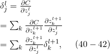
\delta^l_j & = & \frac{\partial C}{\partial z^l_j} \tag{40}\\ & = & \sum_k \frac{\partial C}{\partial z^{l+1}_k} \frac{\partial z^{l+1}_k}{\partial z^l_j} \tag{41}\\ & = & \sum_k \frac{\partial z^{l+1}_k}{\partial z^l_j} \delta^{l+1}_k, \ \ \ \ (40 - 42)

……

where in the last line we have interchanged the two terms on the right-hand side, and substituted the definition of \delta^{l+1}_k. To evaluate the first term on the last line, note that

z^{l+1}_k = \sum_j w^{l+1}_{kj} a^l_j +b^{l+1}_k = \sum_j w^{l+1}_{kj} \sigma(z^l_j) +b^{l+1}_k. \ \ \ \ (43)

Differentiating, we obtain

\frac{\partial z^{l+1}_k}{\partial z^l_j} = w^{l+1}_{kj} \sigma'(z^l_j). \ \ \ \ (44)

Substituting back into (42) we obtain

\delta^l_j = \sum_k w^{l+1}_{kj} \delta^{l+1}_k \sigma'(z^l_j). \ \ \ \ (45)

This is just (BP2) written in component form.

───


或許僅需補之以『推演示意』︰

Derivation

Since backpropagation uses the gradient descent method, one needs to calculate the derivative of the squared error function with respect to the weights of the network. Assuming one output neuron,[note 2] the squared error function is:

E = \tfrac{1}{2}(t - y)^2,

where

E is the squared error,
t is the target output for a training sample, and
y is the actual output of the output neuron.

The factor of \textstyle\frac{1}{2} is included to cancel the exponent when differentiating. Later, the expression will be multiplied with an arbitrary learning rate, so that it doesn’t matter if a constant coefficient is introduced now.

For each neuron j, its output o_{j} is defined as

o_{j} = \varphi(\mbox{net}_{j}) = \varphi\left(\sum_{k=1}^{n}w_{kj}o_k\right).

The input \mbox{net}_{j} to a neuron is the weighted sum of outputs o_k of previous neurons. If the neuron is in the first layer after the input layer, the o_k of the input layer are simply the inputs x_k to the network. The number of input units to the neuron is n. The variable w_{ij} denotes the weight between neurons i and j.

The activation function \varphi is in general non-linear and differentiable. A commonly used activation function is the logistic function:

 \varphi(z) = \frac{1}{1+e^{-z}}

which has a nice derivative of:

 \frac {d \varphi}{d z}(z) = \varphi(z)(1-\varphi(z))

Finding the derivative of the error

Calculating the partial derivative of the error with respect to a weight w_{ij} is done using the chain rule twice:

\frac{\partial E}{\partial w_{ij}} = \frac{\partial E}{\partial o_j} \frac{\partial o_j}{\partial\mathrm{net_j}} \frac{\partial \mathrm{net_j}}{\partial w_{ij}}

In the last term of the right-hand side of the following, only one term in the sum \mathrm{net_j} depends on w_{ij}, so that

\frac{\partial \mathrm{net_j}}{\partial w_{ij}} = \frac{\partial}{\partial w_{ij}}\left(\sum_{k=1}^{n}w_{kj}o_k\right) = o_i.

If the neuron is in the first layer after the input layer, o_i is just x_i.

The derivative of the output of neuron j with respect to its input is simply the partial derivative of the activation function (assuming here that the logistic function is used):

\frac{\partial o_j}{\partial\mathrm{net_j}} = \frac {\partial}{\partial \mathrm{net_j}}\varphi(\mathrm{net_j}) = \varphi(\mathrm{net_j})(1-\varphi(\mathrm{net_j}))

This is the reason why backpropagation requires the activation function to be differentiable.

The first term is straightforward to evaluate if the neuron is in the output layer, because then o_j = y and

\frac{\partial E}{\partial o_j} = \frac{\partial E}{\partial y} = \frac{\partial}{\partial y} \frac{1}{2}(t - y)^2 = y - t

However, if j is in an arbitrary inner layer of the network, finding the derivative E with respect to o_j is less obvious.

Considering E as a function of the inputs of all neurons L = {u, v, \dots, w} receiving input from neuron j,

\frac{\partial E(o_j)}{\partial o_j} = \frac{\partial E(\mathrm{net}_u, \mathrm{net}_v, \dots, \mathrm{net}_w)}{\partial o_j}

and taking the total derivative with respect to o_j, a recursive expression for the derivative is obtained:

\frac{\partial E}{\partial o_j} = \sum_{l \in L} \left(\frac{\partial E}{\partial \mathrm{net}_l}\frac{\partial \mathrm{net}_l}{\partial o_j}\right) = \sum_{l \in L} \left(\frac{\partial E}{\partial o_{l}}\frac{\partial o_{l}}{\partial \mathrm{net}_l}w_{jl}\right)

Therefore, the derivative with respect to o_j can be calculated if all the derivatives with respect to the outputs o_l of the next layer – the one closer to the output neuron – are known.

Putting it all together:

\dfrac{\partial E}{\partial w_{ij}} = \delta_{j} o_{i}

with

\delta_{j} = \frac{\partial E}{\partial o_j} \frac{\partial o_j}{\partial\mathrm{net_j}} = \begin{cases} (o_{j}-t_{j})o_{j}(1-o_{j}) & \mbox{if } j \mbox{ is an output neuron,}\\ (\sum_{l\in L} \delta_{l} w_{jl})o_{j}(1-o_{j}) & \mbox{if } j \mbox{ is an inner neuron.} \end{cases}

To update the weight w_{ij} using gradient descent, one must choose a learning rate, \alpha. The change in weight, which is added to the old weight, is equal to the product of the learning rate and the gradient, multiplied by -1:

 \Delta w_{ij} = - \alpha \frac{\partial E}{\partial w_{ij}} = \begin{cases} - \alpha o_{i} (o_{j}-t_{j})o_{j}(1-o_{j}) & \mbox{if } j \mbox{ is an output neuron,}\\ - \alpha o_{i} (\sum_{l\in L} \delta_{l} w_{jl})o_{j}(1-o_{j}) & \mbox{if } j \mbox{ is an inner neuron.} \end{cases}

The \textstyle -1 is required in order to update in the direction of a minimum, not a maximum, of the error function.

For a single-layer network, this expression becomes the Delta Rule. To better understand how backpropagation works, here is an example to illustrate it: The Back Propagation Algorithm, page 20.

───


終必得到乎??!!


W!o+ 的《小伶鼬工坊演義》︰神經網絡【backpropagation】七

為什麼一個演算法之『計算速度』值得大書特書的呢??

In what sense is backpropagation a fast algorithm?

In what sense is backpropagation a fast algorithm? To answer this question, let’s consider another approach to computing the gradient. Imagine it’s the early days of neural networks research. Maybe it’s the 1950s or 1960s, and you’re the first person in the world to think of using gradient descent to learn! But to make the idea work you need a way of computing the gradient of the cost function. You think back to your knowledge of calculus, and decide to see if you can use the chain rule to compute the gradient. But after playing around a bit, the algebra looks complicated, and you get discouraged. So you try to find another approach. You decide to regard the cost as a function of the weights C = C(w) alone (we’ll get back to the biases in a moment). You number the weights w_1, w_2, \ldots and want to compute \partial C / \partial w_j for some particular weight w_j. An obvious way of doing that is to use the approximation

C}{\partial w_{j}} \approx \frac{C(w+\epsilon e_j)-C(w)}{\epsilon}, \ \ \ \ (46)

where \epsilon > 0 is a small positive number, and e_j is the unit vector in the j^{\rm th} direction. In other words, we can estimate \partial C / \partial w_j by computing the cost C for two slightly different values of w_j, and then applying Equation (46). The same idea will let us compute the partial derivatives \partial C / \partial b with respect to the biases.

This approach looks very promising. It’s simple conceptually, and extremely easy to implement, using just a few lines of code. Certainly, it looks much more promising than the idea of using the chain rule to compute the gradient!

Unfortunately, while this approach appears promising, when you implement the code it turns out to be extremely slow. To understand why, imagine we have a million weights in our network. Then for each distinct weight w_j we need to compute C(w+\epsilon e_j) in order to compute \partial C / \partial w_j. That means that to compute the gradient we need to compute the cost function a million different times, requiring a million forward passes through the network (per training example). We need to compute C(w) as well, so that’s a total of a million and one passes through the network.

What’s clever about backpropagation is that it enables us to simultaneously compute all the partial derivatives \partial C / \partial w_j using just one forward pass through the network, followed by one backward pass through the network. Roughly speaking, the computational cost of the backward pass is about the same as the forward pass*

*This should be plausible, but it requires some analysis to make a careful statement. It’s plausible because the dominant computational cost in the forward pass is multiplying by the weight matrices, while in the backward pass it’s multiplying by the transposes of the weight matrices. These operations obviously have similar computational cost..

And so the total cost of backpropagation is roughly the same as making just two forward passes through the network. Compare that to the million and one forward passes we needed for the approach based on (46)! And so even though backpropagation appears superficially more complex than the approach based on (46), it’s actually much, much faster.

This speedup was first fully appreciated in 1986, and it greatly expanded the range of problems that neural networks could solve. That, in turn, caused a rush of people using neural networks. Of course, backpropagation is not a panacea. Even in the late 1980s people ran up against limits, especially when attempting to use backpropagation to train deep neural networks, i.e., networks with many hidden layers. Later in the book we’ll see how modern computers and some clever new ideas now make it possible to use backpropagation to train such deep neural networks.

───


因為『實務機器』是『受限的』 bounded ,所以講『記憶體』、『輸出入快慢』、『CPU 速度』…… 都是『有限資源』!?如果說對比『理論之圖靈機』,它的『讀寫磁帶』是『無限的』!它的『狀態變遷速度』是無關緊要的!!

因此假使從『無限長』 \infty 之天外時間來看, 2^{1024} 年是否算久的呢 ??!!要是自『人的壽限』觀之 ,怕連 2^8 年都捱不了的吧!! ??此即是『正寫』為什麼人總得談那個『速度』的哩!!!或許這時『反思』『自然創造』,生物之『成長學習』卻一直是『按部就班』,豈不令人驚奇的耶???

如何直觀『反向傳播演算法』之『速度』的乎?偶讀 colah’s blog 之文章 ,心想有益且介紹給讀者︰

Calculus on Computational Graphs: Backpropagation

Posted on August 31, 2015

Introduction

Backpropagation is the key algorithm that makes training deep models computationally tractable. For modern neural networks, it can make training with gradient descent as much as ten million times faster, relative to a naive implementation. That’s the difference between a model taking a week to train and taking 200,000 years.

Beyond its use in deep learning, backpropagation is a powerful computational tool in many other areas, ranging from weather forecasting to analyzing numerical stability – it just goes by different names. In fact, the algorithm has been reinvented at least dozens of times in different fields (see Griewank (2010)). The general, application independent, name is “reverse-mode differentiation.”

Fundamentally, it’s a technique for calculating derivatives quickly. And it’s an essential trick to have in your bag, not only in deep learning, but in a wide variety of numerical computing situations.

……

Conclusion

Derivatives are cheaper than you think. That’s the main lesson to take away from this post. In fact, they’re unintuitively cheap, and us silly humans have had to repeatedly rediscover this fact. That’s an important thing to understand in deep learning. It’s also a really useful thing to know in other fields, and only more so if it isn’t common knowledge.

Are there other lessons? I think there are.

Backpropagation is also a useful lens for understanding how derivatives flow through a model. This can be extremely helpful in reasoning about why some models are difficult to optimize. The classic example of this is the problem of vanishing gradients in recurrent neural networks.

Finally, I claim there is a broad algorithmic lesson to take away from these techniques. Backpropagation and forward-mode differentiation use a powerful pair of tricks (linearization and dynamic programming) to compute derivatives more efficiently than one might think possible. If you really understand these techniques, you can use them to efficiently calculate several other interesting expressions involving derivatives. We’ll explore this in a later blog post.

This post gives a very abstract treatment of backpropagation. I strongly recommend reading Michael Nielsen’s chapter on it for an excellent discussion, more concretely focused on neural networks.

───


由於作者不知那個『反向傳播演算法』之『大數趨近行為』 Big O notation

大O符號

大O符號英語:Big O notation)是用於描述函數漸近行為數學符號。更確切地說,它是用另一個(通常更簡單的)函數來描述一個函數數量級漸近上界。在數學中,它一般用來刻畫被截斷的無窮級數尤其是漸近級數的剩餘項;在計算機科學中,它在分析算法複雜性的方面非常有用。

大O符號是由德國數論學家保羅·巴赫曼(Paul Bachmann)在其1892年的著作《解析數論》(Analytische Zahlentheorie)首先引入的。而這個記號則是在另一位德國數論學家艾德蒙·朗道(Edmund Landau)的著作中才推廣的,因此它有時又稱為朗道符號(Landau symbols)。代表「order of …」(……階)的大O,最初是一個大寫的希臘字母Ο‘(omicron),現今用的是大寫拉丁字母O』,但從來不是阿拉伯數字『0』

───

f(x) \equiv O(g(x)) , \ \ \ if \ \ x \to \infty \ \  \frac{f(x)} {g(x)} \approx const.


故而無法多說,僅舉

Fast Fourier transform

A fast Fourier transform (FFT) algorithm computes the discrete Fourier transform (DFT) of a sequence, or its inverse. Fourier analysis converts a signal from its original domain (often time or space) to a representation in the frequency domain and vice versa. An FFT rapidly computes such transformations by factorizing the DFT matrix into a product of sparse (mostly zero) factors.[1] As a result, it manages to reduce the complexity of computing the DFT from O(n^2), which arises if one simply applies the definition of DFT, to O(n \log n), where n is the data size.

Fast Fourier transforms are widely used for many applications in engineering, science, and mathematics. The basic ideas were popularized in 1965, but some algorithms had been derived as early as 1805.[2] In 1994 Gilbert Strang described the FFT as “the most important numerical algorithm of our lifetime”[3] and it was included in Top 10 Algorithms of 20th Century by the IEEE journal Computing in Science & Engineering.[4]

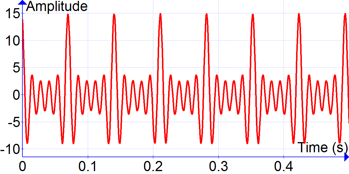
 Time_Signal_of_Five_Term_Cosine_Series
Time signal of a five term cosine series. Frequencies are multiples of 10 times sqrt(2). Amplitudes are 1, 2, 3, 4, 5. Time step is 0.001 s

───


為例講講『速度』重要性。假使 n = {10}^6 ,那麼 O(n^2) 之 DFT 大約需要 {10}^{12} 個計算,然而 O(n \cdot log(n)) 的 DFT 卻只不過要 {10}^6 \cdot 6 個計算,果真天差地別也耶!!??


W!o+ 的《小伶鼬工坊演義》︰神經網絡【backpropagation】六

俗話說︰千里來龍,在此結穴。 Michael Nielsen 先生這段文字

The backpropagation algorithm

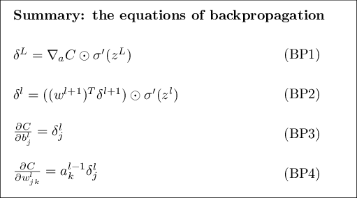
The backpropagation equations provide us with a way of computing the gradient of the cost function. Let’s explicitly write this out in the form of an algorithm:

  1. Input x : Set the corresponding activation a^l for the input layer.
  2. Feedforward: For each l = 2, 3, \ldots, L compute z^{l} = w^l a^{l-1}+b^l and a^{l} = \sigma(z^{l}).
  3. Output error \delta^L : Compute the vector \delta^{L} = \nabla_a C \odot \sigma'(z^L).
  4. Backpropagate the error: For each l = L-1, L-2, \ldots, 2 compute \delta^{l} = ((w^{l+1})^T \delta^{l+1}) \odot \sigma'(z^{l}).
  5. Output: The gradient of the cost function is given by \frac{\partial C}{\partial w^l_{jk}} = a^{l-1}_k \delta^l_j and \frac{\partial C}{\partial b^l_j} = \delta^l_j.

Examining the algorithm you can see why it’s called backpropagation. We compute the error vectors δl backward, starting from the final layer. It may seem peculiar that we’re going through the network backward. But if you think about the proof of backpropagation, the backward movement is a consequence of the fact that the cost is a function of outputs from the network. To understand how the cost varies with earlier weights and biases we need to repeatedly apply the chain rule, working backward through the layers to obtain usable expressions.

……

As I’ve described it above, the backpropagation algorithm computes the gradient of the cost function for a single training example, C = C_x. In practice, it’s common to combine backpropagation with a learning algorithm such as stochastic gradient descent, in which we compute the gradient for many training examples. In particular, given a mini-batch of m training examples, the following algorithm applies a gradient descent learning step based on that mini-batch:

  1. Input a set of training examples
  2. For each training example  x : Set the corresponding input activation a^{x,1, and perform the following steps:
    • Feedforward: For each l = 2, 3, \ldots, L compute z^{x,l} = w^l a^{x,l-1}+b^l and a^{x,l} = \sigma(z^{x,l}).
    • Output error \delta^{x,L} : Compute the vector \delta^{x,L} = \nabla_a C_x \odot \sigma'(z^{x,L}).
    • Backpropagate the error: For each l = L-1, L-2, \ldots, 2 compute \delta^{x,l} = ((w^{l+1})^T \delta^{x,l+1}) \odot \sigma'(z^{x,l}).
  3. Gradient descent: For each l = L, L-1, \ldots, 2 update the weights according to the rule w^l \rightarrow w^l-\frac{\eta}{m} \sum_x \delta^{x,l} (a^{x,l-1})^T, and the biases according to the rule b^l \rightarrow b^l-\frac{\eta}{m} \sum_x \delta^{x,l}.

Of course, to implement stochastic gradient descent in practice you also need an outer loop generating mini-batches of training examples, and an outer loop stepping through multiple epochs of training. I’ve omitted those for simplicity.

───


或許讀來輕鬆快意!就連程式碼

The code for backpropagation

Having understood backpropagation in the abstract, we can now understand the code used in the last chapter to implement backpropagation. Recall from that chapter that the code was contained in the update_mini_batch and backprop methods of the Network class. The code for these methods is a direct translation of the algorithm described above. In particular, the update_mini_batch method updates the Network‘s weights and biases by computing the gradient for the current mini_batch of training examples:

class Network(object):
...
    def update_mini_batch(self, mini_batch, eta):
        """Update the network's weights and biases by applying
        gradient descent using backpropagation to a single mini batch.
        The "mini_batch" is a list of tuples "(x, y)", and "eta"
        is the learning rate."""
        nabla_b = [np.zeros(b.shape) for b in self.biases]
        nabla_w = [np.zeros(w.shape) for w in self.weights]
        for x, y in mini_batch:
            delta_nabla_b, delta_nabla_w = self.backprop(x, y)
            nabla_b = [nb+dnb for nb, dnb in zip(nabla_b, delta_nabla_b)]
            nabla_w = [nw+dnw for nw, dnw in zip(nabla_w, delta_nabla_w)]
        self.weights = [w-(eta/len(mini_batch))*nw 
                        for w, nw in zip(self.weights, nabla_w)]
        self.biases = [b-(eta/len(mini_batch))*nb 
                       for b, nb in zip(self.biases, nabla_b)]


Most of the work is done by the line delta_nabla_b, delta_nabla_w = self.backprop(x, y) which uses the backprop method to figure out the partial derivatives \partial C_x / \partial b^l_j and \partial C_x / \partial w^l_{jk}. The backprop method follows the algorithm in the last section closely. There is one small change – we use a slightly different approach to indexing the layers. This change is made to take advantage of a feature of Python, namely the use of negative list indices to count backward from the end of a list, so, e.g., l[-3] is the third last entry in a list l. The code for backprop is below, together with a few helper functions, which are used to compute the \sigma function, the derivative \sigma', and the derivative of the cost function. With these inclusions you should be able to understand the code in a self-contained way. If something’s tripping you up, you may find it helpful to consult the original description (and complete listing) of the code.

class Network(object):
...
   def backprop(self, x, y):
        """Return a tuple "(nabla_b, nabla_w)" representing the
        gradient for the cost function C_x.  "nabla_b" and
        "nabla_w" are layer-by-layer lists of numpy arrays, similar
        to "self.biases" and "self.weights"."""
        nabla_b = [np.zeros(b.shape) for b in self.biases]
        nabla_w = [np.zeros(w.shape) for w in self.weights]
        # feedforward
        activation = x
        activations = [x] # list to store all the activations, layer by layer
        zs = [] # list to store all the z vectors, layer by layer
        for b, w in zip(self.biases, self.weights):
            z = np.dot(w, activation)+b
            zs.append(z)
            activation = sigmoid(z)
            activations.append(activation)
        # backward pass
        delta = self.cost_derivative(activations[-1], y) * \
            sigmoid_prime(zs[-1])
        nabla_b[-1] = delta
        nabla_w[-1] = np.dot(delta, activations[-2].transpose())
        # Note that the variable l in the loop below is used a little
        # differently to the notation in Chapter 2 of the book.  Here,
        # l = 1 means the last layer of neurons, l = 2 is the
        # second-last layer, and so on.  It's a renumbering of the
        # scheme in the book, used here to take advantage of the fact
        # that Python can use negative indices in lists.
        for l in xrange(2, self.num_layers):
            z = zs[-l]
            sp = sigmoid_prime(z)
            delta = np.dot(self.weights[-l+1].transpose(), delta) * sp
            nabla_b[-l] = delta
            nabla_w[-l] = np.dot(delta, activations[-l-1].transpose())
        return (nabla_b, nabla_w)

...

    def cost_derivative(self, output_activations, y):
        """Return the vector of partial derivatives \partial C_x /
        \partial a for the output activations."""
        return (output_activations-y) 

def sigmoid(z):
    """The sigmoid function."""
    return 1.0/(1.0+np.exp(-z))

def sigmoid_prime(z):
    """Derivative of the sigmoid function."""
    return sigmoid(z)*(1-sigmoid(z))

───


也彷彿一目瞭然!!當此之際,需注意『去脈問題』?一如之前

W!o+ 的《小伶鼬工坊演義》︰神經網絡【Sigmoid】六》文本

所講,這個『Stochastic gradient descent』方法是有『假設前提』的,那個『學習率』 \eta 和『批量值』 m 都是『超參數』,如何適當選取,尚須慎思與明辨耶??

此刻讀點『天外飛來一筆』□○ 之文,或有益乎??!!

在《λ 運算︰淵源介紹》一文中,我們談過『函數y = f(x) = x^2 中的『變數x 是『虛名的』,它是函數『定義域』的『輸入值』,而那個 y 是函數『對應域』之『輸出值』。這個『函數』是由『計算規則\Box^2 來確定的,把它叫做 f(x) 或者 g(w), \ z = g(w) = w^2 都指相同的『函數』,因此『函數』就其『抽象定義』來講是『匿名的』。於是所謂的『命名』也只是方便『指稱』或『分別』不同的『函數』罷了!當一個『函數F 的『定義域』中的『元素h 也是『函數』時,此時就很容易發生了『混淆』,它是指一個『定義域』是『變數x 的『複合函數H = F \circ h, \ H(x) = F(h(x)),還是指『定義域』是『函數h(x)  之『泛函數』 functional 的呢?比方說 H(t) = \int_{0}^{t} h(x) dx,也許最好將此類的『泛函數』稱之為『函式』較好。如此當一個含有『未知函數』或者『隱函數』的『複合函數』之方程式被叫做『 泛函數方程式』Functional equation 時,也就能夠作個清楚『區分』的了!!

那麼『 泛函數方程式』有什麼『重要性』的嗎?就讓我們從一個『例子』開始談吧︰

f(x + y) = f(x) \cdot f(y)

。就是說有個『未知函數f  將『定義域』中『兩數的加法x + y 轉換成了『對應域』裡『兩數之乘法』  f(x) \cdot f(y)。這個『未知函數』的『整體性質』就由這個『方程式』 來決定,比方講,這個函數 f(0) = 1,為什麼呢?因為 f(0) = f(0 + 0) = f(0) \cdot f(0) = {f(0)}^2,所以 f(0) = 0f(0) = 1,又為什麼不取 f(0) = 0 的呢?因為如果取  f(0) = 0 的話,f(x) = f(x + 0) = f(x) \cdot f(0) = 0 只是個『零函數』罷了,一般叫做『平凡解』 trivial solution,雖然它為了『完整性』不能夠『被省略』,然而這個解『太顯然』的了 ── 0 + 0 = 0 \cdot 0,似乎不必『再說明』的吧!不過有時這種『論證』的傳統給『初學者』帶來了『理解』的『困難』,故此特別指出。要怎麼『求解』 泛函數方程式的呢?一般說來『非常困難』,有時甚至可能無法得知它到底是有『一個解』、『多個解』、『無窮解』或者根本就『無解』!!近年來漸漸的產生了一些『常用方法』,比方講『動態規劃』 Dynamic programming 中使用『分割征服』的『連續逼近法』或是將原方程式『變換』成適合『定點迭代法』等等。在此我們將介紹『無窮小分析』的『應用』,談一點對於一個『平滑函數f(x) 來說,可以如何『思考』這種方程式的呢?由於 f(x) 是『平滑的』,因此 f(x) 它『可微分』,『導數f^{\prime}(x) 存在而且『連續』,那麼 f(x + \delta x) 就可以表示為

f(x + \delta x) = f(x) + f^{\prime}(x) \cdot \delta x + \epsilon \cdot \delta x

, 此處 \delta x \approx 0 \Longrightarrow \epsilon \approx 0。由於 f(x + y) = f(x) \cdot f(y),可得 f(x + \delta x) = f(x) \cdot f(\delta x),因此 f(x + \delta x) = f(x) \cdot f(\delta x) = f(x) + f^{\prime}(x) \cdot \delta x + \epsilon \cdot \delta x,所以

\frac{f^{\prime}(x)}{f(x)} = \frac{f(\delta x) - 1}{\delta x} - \epsilon

。因為 f(x) 是『平滑的』,那麼 \frac{f^{\prime}(x)}{f(x)} 將存在且連續,然而 \frac{f(\delta x) - 1}{\delta x} - \epsilon 與『變數x 無關,於是當 \delta x \approx 0 時,必定是某個『常數』 constant ,將之命作 k,如此那個『 泛函數方程式』就被改寫成了『微分方程式

f^{\prime}(x) = k \cdot f(x), \ f(0) = 1

。它的『』是 f(x) = e^{k \cdot x}, \ k \neq 0,為什麼 k \neq 0 的呢?因為此時 f^{\prime}(x) = 0,將會得到 f(x) 是個『常數函數』,這就是前面說的那個『平凡解』 的啊!!

乍一看,這個『解法』果真『奇妙』,竟然變成了『微分方程式』的了!假使細察 f(x + y) = f(x) \cdot f(y) 可說是『函數f(x) 的『大域性質』,但是 f(x + \delta x) = f(x) + f^{\prime}(x) \cdot \delta x + \epsilon \cdot \delta x 卻描述『函數f(x) 之『微觀鄰域』,將此兩者合併考慮,果真是『可以的』嗎?如果說一個函數的『大域性質』自然『含括\Longrightarrow 了它的『微觀鄰域』之『描述』,由於它是一個『平滑的』函數,那麼『微觀鄰域』的『微分方程式』難道不能『整合』 integrate \Longrightarrow 成那個『大域性質』的嗎?

─── 摘自《【Sonic π】電聲學之電路學《四》之《一》


W!o+ 的《小伶鼬工坊演義》︰神經網絡【backpropagation】五

人能否從歷史人物身上學習什麼呢?比方說維基百科『高斯』詞條如是紀載︰

約翰·卡爾·弗里德里希·高斯德語:Johann Karl Friedrich Gauß關於這個音頻文件 

英語:Gauss拉丁語Carolus Fridericus Gauss;1777年4月30日-1855年2月23日), 德國著名數學家物理學家天文學家大地測量學家,生於布倫瑞克,卒於哥廷根 。高斯被認為是歷史上最重要的數學家之一[1],並有「數學王子」的美譽[2]

1792年,15歲的高斯進入Collegium Carolinum,現今的布倫瑞克科技大學(Braunschweig University of Technology)。在那裡,高斯開始對高等數學作研究。獨立發現了二項式定理的一般形式、數論上的「二次互反律」、質數定理、及算術-幾何平均數[3]

1795年高斯進入哥廷根大學。1796年,19歲的高斯得到了一個數學史上極重要的結果,就是《正十七邊形尺規作圖之理論與方法》。

1855年2月23日清晨,77歲的高斯在格於丁根天文台的躺椅上睡覺時去世。[4]

Bendixen_-_Carl_Friedrich_Gauß,_1828

1838年出版的天文學通報中高斯肖像。

生平

高斯是一對普通夫婦的兒子。他的母親是一個貧窮石匠的女兒,雖然十分聰明,但卻沒有接受過教育,近似於文盲。在她成為高斯父親的第二個妻子之前,她從事女傭工作。他的父親曾做過工頭,商人的助手和一個小保險公司的評估師。高斯三歲時便能夠糾正他父親的借債帳目的事情,已經成為一個軼事流傳至今。他曾說,他能夠在腦袋中進行複雜的計算。他的職業是園丁,他做事認真。

高斯10歲時利用很短的時間就計算出了小學老師提出的問題:自然數從1到100的求和。他所使用的方法是:對50對構造成和101的數列求和(1+100,2+99,3+98……),同時得到結果:5050。

───


這位一代之數學天才有著非凡的洞察力!能用不俗的觀點處理數學計算問題!!傳聞所說的老師之刁難︰計算

1+2+3+ \cdots + 99 +100

,終因『巧妙』之法而迅速落幕也︰

Sum = 1+2+3+ \cdots + 99 +100

Sum = 100+99+ \cdots +3+2 +1

2 \cdot Sum = (1+100) + (2+99) + \cdots + (99+2) + (100+1)

= (101) \times 100

\therefore Sum = \frac{101 \times 100}{2} = 5050


但是此『巧妙』之法難以『推廣』,舉例說︰計算

1^2 + 2^2 + 3^2 + \cdots + {99}^2 +{100}^2

無法運作此法也??!!難道還有更『一般性』的法子嗎??假使設想一個『序列』 S_n = n^2 ,可知 S_{n+1} - S_n = {(n+1)}^2 - n^2 = 2 \cdot n +1 ,因此

S_2 - S_1 = 2 \cdot 1 +1

S_3 - S_2 = 2 \cdot 2 +1

……

S_n - S_{n-1} = 2 \cdot (n-1) + 1

S_{n+1} - S_n = 2 \cdot n +1

\therefore S_{n+1} - S_1 = 2 \cdot (1+2+ \cdots + (n-1) + n) + n

所以

1+2+ \cdots + (n-1) + n = \frac{S_{n+1} - S_1 - n}{2} = \frac{n \cdot (n+1)} {2}


要是依樣畫葫蘆構造『序列』 C_n = n^3 , 那麼 C_{n+1} - C_n = {(n+1)}^3 - n^3 = 3 \cdot n^2 + 3 \cdot n + 1 ,故而

C_2 - C_1 = 3 \cdot 1^2 + 3 \cdot 1 +1

C_3 - C_2 = 3 \cdot 2^2 + 3 \cdot 2 +1

……

C_n - C_{n-1} = 3 \cdot {(n-1)}^2 + 3 \cdot (n-1) +1

C_{n+1} - C_n = 3 \cdot n^2 + 3 \cdot n +1

\therefore C_{n+1} - C_1 = 3 \cdot (1^2 + 2^2 + \cdots + n^2) + 3 \cdot (1+2+ \cdots +n) + n

於是

1^2 + 2^2 + \cdots + n^2 = \frac{C_{n+1} - C_1 - 3 \cdot (1+2+ \cdots +n) - n}{3} = \frac{n \cdot (n+1) \cdot (2 \cdot n +1)}{6}


果真可以『類推』耶!!??反之我們曉得 1^2 + 2^2 + \cdots + n^2 必為整數,因此 n \cdot (n+1) \cdot (2 \cdot n +1) 必是六的倍數,但將要如何證明的呢???故知方法有窮而無盡!應用無窮實難盡!!終究運作之道祇存乎一心矣!!!

作者之所以寫這一段前言,是想說明『反向傳播演算法』不外乎是依據『定義』

\delta^l_j \equiv \frac{\partial C}{\partial z^l_j}. \ \ \ \ (29)

,使用『鏈式法則』有『目的』之『推導』罷了??

tikz21


如能清清楚楚了解此『目的』,『推導』方向的『選擇』也就明明白白,不欲做『多餘之計算』也!從『已知』推向『未知』的呀 !!

層與層之間有關係

{\vec z}^{\ l} \ \equiv \  W^{\ l} \ {\vec a}^{\ l-1}  \ + \ {\vec b}^{\ l}

可以『向前瞧』或『向後看』,既然名之為『反向』欲『向後看』也。為什麼的呢?因為我們僅知『最終誤差』是

C = \frac{1}{2n} \sum_x \|y(x)-a^L(x)\|^2, \ \ \ \ (26)

,我們想透過改變『之前』的『權重』W^{\ l}  和『基底』 {\vec b} ^l 來『減少』此『誤差』,『向後看』才能知道將改變多少的乎!!

因此當 Michael Nielsen 先生證明式子 BP2 時,首先明示此『目的』

Next, we’ll prove (BP2), which gives an equation for the error \delta^l in terms of the error in the next layer, \delta^{l+1}. To do this, we want to rewrite \delta^l_j = \partial C / \partial z^l_j in terms of \delta^{l+1}_k = \partial C / \partial z^{l+1}_k. We can do this using the chain rule,

\delta^l_j & = & \frac{\partial C}{\partial z^l_j} \tag{40}\\ & = & \sum_k \frac{\partial C}{\partial z^{l+1}_k} \frac{\partial z^{l+1}_k}{\partial z^l_j} \tag{41}\\ & = & \sum_k \frac{\partial z^{l+1}_k}{\partial z^l_j} \delta^{l+1}_k, \ \ \ \ (40 - 42)
───


,實是畫龍點睛之筆法也。

由於 BP3 、BP4 兩式之證明給當成了『習題』,此處就算『題解』的吧。為方便閱讀,列出相干關係函式如下︰

C = C({\vec a}^L)

{\vec a}^L = \sigma ({\vec z}^L)

\sigma(z) \equiv \frac{1}{1+e^{-z}}

{\vec z}^{\ l} \ \equiv \  W^{\ l} \ {\vec a}^{\ l-1}  \ + \ {\vec b}^{\ l}

\delta^l_j \equiv \frac{\partial C}{\partial z^l_j}. \ \ \ \ (29)


【BP3】

\frac{\partial C}{\partial b^l_j} = \frac{\partial C}{\partial z^l_j}  \cdot \frac{\partial z^l_j}{\partial b^l_j} = \delta^l_j \cdot 1 = \delta^l_j


【BP4】

\frac{\partial C}{\partial w^l_{jk}} = \frac{\partial C}{\partial z^l_j} \cdot \frac{\partial z^l_j}{\partial w^l_{jk}} = \delta^l_j \cdot a^{l-1}_k = a^{l-1}_k \cdot \delta^l_j