仔細考察一個典型統計問題︰

人類身高

身高，又稱身長，是指一個人從頭頂到腳底的身體長度。

成年人的身高有一個標準範圍，並且在同民族同性別內部遵循常態分布。身高的標準範圍可以用常態分布中的標準差（σ）定義的z-score衡量^[1]：

z =（身高-參考組身高中間值）/σ

一般差出 2-3σ（對成人 3σ 大致相當於與平均身高差到20%）的被認為是反常身高，例如巨人症或侏儒症患者；但反常身高本身不一定在醫學上被視為疾病。

因為站立行走時體重對脊椎的壓縮，成年人一天之內的身高變化平均可達 1.9公分（0.75英寸）

身高的形成

人的一生中，身體增長最快的有兩個階段：出生至1歲，和青春期期間。青春期後期至20歲初達到成年身高。成年身高由先天基因和後天環境因素決定。

最優環境下的人體生長速度曲線(Courtesy: Richard Steckel)

基因在個人身高的決定中占重要地位。無明顯外因的身材矮小，包括病態的生長激素分泌不足情況，可以給與提煉或人工合成的生長激素。但這類治療價格昂貴，而且很多人認為這更加重了身高歧視，不贊成對個子矮但無其他發育缺陷的兒童使用生長激素。

一個人群的平均身高則和環境因素，特別是兒童時期的健康和營養情況更有關。患病、感染、飢餓、貧血、缺乏蛋白質、缺乏鈣、鋅等元素，都會妨礙身高增長。由於現代醫學和農業的進步，已開發國家和富裕的開發中國家人口身高都比歷史上有不同程度的增長。現在朝鮮的青年人平均比韓國矮8厘米，主要是前者近年來饑饉的結果。再例如在19世紀初，英國工業革命造成廣泛污染和生活環境不良的時候，人口平均身高達到了歷史最低點時，比其前（農業社會）和其後（福利工業社會）都要低。

影響身高的因素

影響身高的主要原因大概有以下幾種：

遺傳：大多個子比較高父母的小孩通常比較高；個子矮的則比較矮，但只是其一因素，如小孩在其他部份條件良好，成長後也會有一定的身高。
營養：鈣質、維生素D及蛋白質是最影響人類身高的營養，這對身高影響非常大，很多先天因素良好的人因營養不良而長得不太高。
運動：運動能刺激食慾低的小個子，使其能補充營養，如為高動物蛋白高鈣可長高，其他高熱量則無效。
睡眠：因腦下垂體只會在人類睡覺時產生生長激素，因此影響身高。
發育：發育的先後非常影響人類的身高，女生一般較男生矮小是因為女性一般較早發育，這也是為什么小學時期女生會比男生高的原因。但因男生的發育時間較後，所以一個條件一般的男生最晚會在高中時比一個條件優秀的女生高。男可比父母較高的一方高至多25厘米，女可比父母較矮的一方高至多25厘米，而早熟跟晚熟也會有身高的分別，一個晚熟的男生可能十四歲至十六歲時才開始發育，因為他的長高時間較長（一般男生長高的時間大概是20年左右），所以在後期會比早熟的還要高。

身高的變化

一個人的身高剛起床時比入睡時高出兩厘米，這是因為日間直立的姿勢壓縮椎間盤，而睡眠時椎間盤得到放鬆恢復原有高度。躺著量頭到腳的長度也會比站著量多出2.54厘米。太空人們在失重的狀態下會增高5-7厘米，回到地球後會逐漸恢復到原有高度。

人類的平均身高並非是一成不變的，科學界普遍認為6000年前農業社會的形成與漁獵的生活方式被農耕取代，造成了人類平均身高的下降，土耳其境內8000年前遺蹟所留下的屍骨平均身高超過今日土耳其的平均身高。　^[2]英國牛津大學里查德教授在分析了幾千具從丹麥、瑞典、挪威、英國和冰島挖掘出來的古代人類男性的遺骨後發現，人類成年男性平均身高在中世紀期間的公元9世紀到12世紀之間到達了一個自10萬年前現代智人誕生以來到20世紀中期前的平均最大值，平均身高為1.73米，然後逐漸變矮變低，到了工業革命前夕的18世紀和19世紀，歐洲成年男性平均身高降低到 1.67米，比9世紀到12世紀間減小了6厘米之多。一直到了20世紀中期，人類男性平均身高才重新恢復達到9世紀到12世紀的最大值。羅馬帝國時期的遺址赫庫蘭尼姆城（在今土耳其境內）前後共出土了近二百餘具遺骸，美國史密森大學物理考古學家薩拉·比西爾對他們進行了深入細緻的研究，了解到古羅馬男子一般身高一點七米，女子一點五五米」。雖然人類的身高在農耕時代後就降至170公分左右，但從1920年開始，特別是從20世紀中期以後，人類平均身高迅速增長，這主要是因為現代蛋白質基礎的食物（蛋、奶、肉）有能力充足供應的關係，歐洲成年男子平均身高從167厘米增長到177厘米，其中比利時成年男子的平均身高從1920年的166厘米增長到1970年的174厘米，丹麥則從169厘米增加到178厘米。^[3]

好好想想可能疑慮︰

Average height around the world

As with any statistical data, the accuracy of such data may be questionable for various reasons:

Some studies may allow subjects to self-report values. Generally speaking, self-reported height tends to be taller than its measured height, although the overestimation of height depends on the reporting subject’s height, age, gender and region.^[61]^[62]^[63]^[64]
Test subjects may have been invited instead of chosen at random, resulting in sampling bias.
Some countries may have significant height gaps between different regions. For instance, one survey shows there is 10.8 cm (4 ¹⁄₂ in) gap between the tallest state and the shortest state in Germany.^[65] Under such circumstances, the mean height may not represent the total population unless sample subjects are appropriately taken from all regions with using weighted average of the different regional groups.
Different social groups can show different mean height. According to a study in France, executives and professionals are 2.6 cm (1 in) taller, and university students are 2.55 cm (1 in) taller^[66] than the national average.^[67]As this case shows, data taken from a particular social group may not represent a total population in some countries.
A relatively small sample of the population may have been measured, which makes it uncertain whether this sample accurately represents the entire population.
The height of persons can vary over the course of a day, due to factors such as a height increase from exercise done directly before measurement (normally inversely correlated), or a height increase since lying down for a significant period of time (normally inversely correlated). For example, one study revealed a mean decrease of 1.54 centimetres (0.61 in) in the heights of 100 children from getting out of bed in the morning to between 4 and 5 p.m. that same day.^[68] Such factors may not have been controlled in some of the studies.
Men from Bosnia and Herzegovina, the Netherlands, Croatia, Serbia, and Montenegro have the tallest average height.^[69]^[70] Data suggests that Herzegovinians have the genetic potential to be more than two inches taller than the Dutch. In the Netherlands, about 35% of men have the genetic profile Y haplogroup I-M170, but in Herzegovina, the frequency is over 70%. Extrapolating the genetic trend line suggests that the average Herzegovinian man could possibly be as tall as 190 cm (nearly 6′ 3″). Many Herzegovinians do not achieve this potential due to poverty (citizens of Bosnia and Herzegovina were 1.9 cm taller if both of their parents went to university, which is considered as a wealth indicator) and to nutritional choices: religious prohibition on pork may be largely to blame for the shorter average stature of Muslim Herzegovinians.^[71]

認真認識每個字詞︰

Normal distribution

In probability theory, the normal (or Gaussian or Gauss or Laplace–Gauss) distribution is a very common continuous probability distribution. Normal distributions are important in statistics and are often used in the natural and social sciences to represent real-valued random variables whose distributions are not known.^[1]^[2] A random variable with a Gaussian distribution is said to be normally distributed and is called a normal deviate.

The normal distribution is useful because of the central limit theorem. In its most general form, under some conditions (which include finite variance), it states that averages of samples of observations of random variables independently drawn from independent distributions converge in distribution to the normal, that is, become normally distributed when the number of observations is sufficiently large. Physical quantities that are expected to be the sum of many independent processes (such as measurement errors) often have distributions that are nearly normal.^[3] Moreover, many results and methods (such as propagation of uncertainty and least squares parameter fitting) can be derived analytically in explicit form when the relevant variables are normally distributed.

The normal distribution is sometimes informally called the bell curve. However, many other distributions are bell-shaped (such as the Cauchy, Student’s t, and logistic distributions).

The probability density of the normal distribution is

$\displaystyle f(x\mid \mu ,\sigma ^{2})={\frac {1}{\sqrt {2\pi \sigma ^{2}}}}e^{-{\frac {(x-\mu )^{2}}{2\sigma ^{2}}}}$

where

$\displaystyle \mu$ is the mean or expectation of the distribution (and also its median and mode),
$\displaystyle \sigma$ is the standard deviation, and
$\displaystyle \sigma ^{2}$ is the variance.

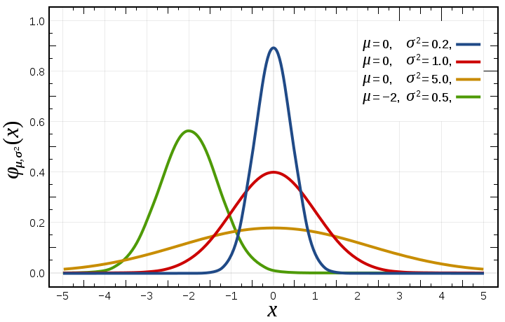
The red curve is the standard normal distribution

充分明白

測量尺度

測量尺度（scale of measure）或稱度量水平（level of measurement）、度量類別，是統計學和定量研究中，對不同種類的數據，依據其尺度水平所劃分的類別，這些尺度水平分別為：名目（nominal）、次序（ordinal）、等距（interval）、等比（ratio）。

名目尺度和次序尺度是定性的，而等距尺度和等比尺度是定量的。定量數據，又根據數據是否可數，分為離散的和連續的。

綜覽

水平	名稱	又稱	可用的邏輯與數學運算方式	舉例	中間趨勢的計算	離散趨勢的計算	定性或定量
1	名目	名義、類別	等於、不等於	二元名目：性別（男、女）二元名目：出席狀況（出席、缺席）二元名目：真實性（真、假）多元名目：語言（中、英、日、法、德文等）多元名目：上市公司（蘋果、美孚、中國石油、沃爾瑪、雀巢等）	眾數	無	定性
2	次序	順序、序列、等級	等於、不等於大於、小於	多元次序：服務評等（傑出、好、欠佳）多元次序：教育程度（小學、初中、高中、學士、碩士、博士等）	眾數、中位數	分位數	定性
3	等距	間隔、區間	等於、不等於大於、小於加、減	溫度、年份、緯度等	眾數、中位數、算術平均數	分位數、全距	定量
4	等比	比率、比例	等於、不等於大於、小於加、減乘、除	價格、年齡、高度、絕對溫度、絕大多數物理量	眾數、中位數、算術平均數、幾何平均數、調和平均數等	分位數、全距、標準差、變異係數等	定量

努力探索背後原理︰

Central limit theorem

In probability theory, the central limit theorem (CLT) establishes that, in some situations, when independent random variables are added, their properly normalized sum tends toward a normal distribution (informally a “bell curve“) even if the original variables themselves are not normally distributed. The theorem is a key concept in probability theory because it implies that probabilistic and statistical methods that work for normal distributions can be applicable to many problems involving other types of distributions.

For example, suppose that a sample is obtained containing a large number of observations, each observation being randomly generated in a way that does not depend on the values of the other observations, and that the arithmetic average of the observed values is computed. If this procedure is performed many times, the central limit theorem says that the computed values of the average will be distributed according to a normal distribution. A simple example of this is that if one flips a coin many times the probability of getting a given number of heads in a series of flips will approach a normal curve, with mean equal to half the total number of flips in each series. (In the limit of an infinite number of flips, it will equal a normal curve.)

The central limit theorem has a number of variants. In its common form, the random variables must be identically distributed. In variants, convergence of the mean to the normal distribution also occurs for non-identical distributions or for non-independent observations, given that they comply with certain conditions.

The earliest version of this theorem, that the normal distribution may be used as an approximation to the binomial distribution, is now known as the de Moivre–Laplace theorem.

In more general usage, a central limit theorem is any of a set of weak-convergence theorems in probability theory. They all express the fact that a sum of many independent and identically distributed (i.i.d.) random variables, or alternatively, random variables with specific types of dependence, will tend to be distributed according to one of a small set of attractor distributions. When the variance of the i.i.d. variables is finite, the attractor distribution is the normal distribution. In contrast, the sum of a number of i.i.d. random variables with power law tail distributions decreasing as $| x | - α - 1$ where $0 < α < 2$ (and therefore having infinite variance) will tend to an alpha-stable distribution with stability parameter (or index of stability) of $α$ as the number of variables grows.^[1]

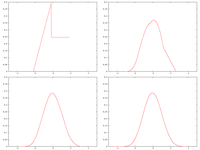
A distribution being “smoothed out” by summation, showing original density of distribution and three subsequent summations; see Illustration of the central limit theorem for further details.

Illustration of the discrete case

This section illustrates the central limit theorem via an example for which the computation can be done quickly by hand on paper, unlike the more computing-intensive example of the previous section.

Original probability mass function

Suppose the probability distribution of a discrete random variable X puts equal weights on 1, 2, and 3:

$\displaystyle X=\left\{{\begin{matrix}1&{\mbox{with}}\ {\mbox{probability}}\ 1/3,\\2&{\mbox{with}}\ {\mbox{probability}}\ 1/3,\\3&{\mbox{with}}\ {\mbox{probability}}\ 1/3.\end{matrix}}\right.$

The probability mass function of the random variable X may be depicted by the following bar graph:

    o    o    o
   -------------
    1    2    3

Clearly this looks nothing like the bell-shaped curve of the normal distribution. Contrast the above with the depictions below.

Probability mass function of the sum of two terms

Now consider the sum of two independent copies of X:

$\displaystyle \left\{{\begin{matrix}1+1&=&2\\1+2&=&3\\1+3&=&4\\2+1&=&3\\2+2&=&4\\2+3&=&5\\3+1&=&4\\3+2&=&5\\3+3&=&6\end{matrix}}\right\}=\left\{{\begin{matrix}2&{\mbox{with}}\ {\mbox{probability}}\ 1/9\\3&{\mbox{with}}\ {\mbox{probability}}\ 2/9\\4&{\mbox{with}}\ {\mbox{probability}}\ 3/9\\5&{\mbox{with}}\ {\mbox{probability}}\ 2/9\\6&{\mbox{with}}\ {\mbox{probability}}\ 1/9\end{matrix}}\right\}$

The probability mass function of this sum may be depicted thus:

              o
         o    o    o
    o    o    o    o    o
   ----------------------------
    2    3    4    5    6

This still does not look very much like the bell-shaped curve, but, like the bell-shaped curve and unlike the probability mass function of X itself, it is higher in the middle than in the two tails.

Probability mass function of the sum of three terms

Now consider the sum of three independent copies of this random variable:

$\displaystyle \left\{{\begin{matrix}1+1+1&=&3\\1+1+2&=&4\\1+1+3&=&5\\1+2+1&=&4\\1+2+2&=&5\\1+2+3&=&6\\1+3+1&=&5\\1+3+2&=&6\\1+3+3&=&7\\2+1+1&=&4\\2+1+2&=&5\\2+1+3&=&6\\2+2+1&=&5\\2+2+2&=&6\\2+2+3&=&7\\2+3+1&=&6\\2+3+2&=&7\\2+3+3&=&8\\3+1+1&=&5\\3+1+2&=&6\\3+1+3&=&7\\3+2+1&=&6\\3+2+2&=&7\\3+2+3&=&8\\3+3+1&=&7\\3+3+2&=&8\\3+3+3&=&9\end{matrix}}\right\}=\left\{{\begin{matrix}3&{\mbox{with}}\ {\mbox{probability}}\ 1/27\\4&{\mbox{with}}\ {\mbox{probability}}\ 3/27\\5&{\mbox{with}}\ {\mbox{probability}}\ 6/27\\6&{\mbox{with}}\ {\mbox{probability}}\ 7/27\\7&{\mbox{with}}\ {\mbox{probability}}\ 6/27\\8&{\mbox{with}}\ {\mbox{probability}}\ 3/27\\9&{\mbox{with}}\ {\mbox{probability}}\ 1/27\end{matrix}}\right\}$

The probability mass function of this sum may be depicted thus:

                   o
              o    o    o
              o    o    o
              o    o    o
         o    o    o    o    o
         o    o    o    o    o
    o    o    o    o    o    o    o
   ---------------------------------
    3    4    5    6    7    8    9

Not only is this bigger at the center than it is at the tails, but as one moves toward the center from either tail, the slope first increases and then decreases, just as with the bell-shaped curve.

The degree of its resemblance to the bell-shaped curve can be quantified as follows. Consider

Pr(X₁ + X₂ + X₃ ≤ 7) = 1/27 + 3/27 + 6/27 + 7/27 + 6/27 = 23/27 = 0.85185… .

How close is this to what a normal approximation would give? It can readily be seen that the expected value of Y = X₁ + X₂ + X₃ is 6 and the standard deviation of Y is the square root of 2. Since Y ≤ 7 (weak inequality) if and only if Y < 8 (strict inequality), we use a continuity correction and seek

$\displaystyle {\mbox{Pr}}(Y\leq 7.5)={\mbox{P}}\left({Y-6 \over {\sqrt {2}}}\leq {7.5-6 \over {\sqrt {2}}}\right)={\mbox{Pr}}(Z\leq 1.0606602\dots )=0.85558\dots$

where Z has a standard normal distribution. The difference between 0.85185… and 0.85558… seems remarkably small when it is considered that the number of independent random variables that were added was only three.

Probability mass function of the sum of 1,000 terms

The following image shows the result of a simulation based on the example presented in this page. The extraction from the uniform distribution is repeated 1,000 times, and the results are summed.

Since the simulation is based on the Monte Carlo method, the process is repeated 10,000 times. The results shows that the distribution of the sum of 1,000 uniform extractions resembles the bell-shaped curve very well.

……

何理不可得也耶？

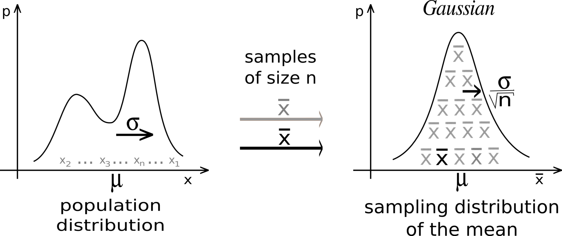
Whatever the form of the population distribution, the sampling distribution tends to a Gaussian, and its dispersion is given by the Central Limit Theorem.^[2]

Independent sequences

Classical CLT

Let ${X 1, \dots, X n}$ be a random sample of size $n$ — that is, a sequence of independent and identically distributed random variables drawn from a distribution of expected value given by $µ$ and finitevariance given by $σ 2$ . Suppose we are interested in the sample average

$\displaystyle S_{n}:={\frac {X_{1}+\cdots +X_{n}}{n}}$

of these random variables. By the law of large numbers, the sample averages converge in probability and almost surely to the expected value

µ

n \to \infty

. The classical central limit theorem describes the size and the distributional form of the stochastic fluctuations around the deterministic number

µ

during this convergence. More precisely, it states that as

n

gets larger, the distribution of the difference between the sample average

S n

and its limit

µ

, when multiplied by the factor

\sqrt n

(that is

\sqrt n (S n - µ)

), approximates the normal distribution with mean 0 and variance

σ 2

. For large enough

n

, the distribution of

S n

is close to the normal distribution with mean

µ

and variance

σ 2 / n

. The usefulness of the theorem is that the distribution of

\sqrt n (S n - µ)

approaches normality regardless of the shape of the distribution of the individual

X i

. Formally, the theorem can be stated as follows:

Lindeberg–Lévy CLT. Suppose ${X 1, X 2, \dots}$ is a sequence of i.i.d. random variables with $E[X i] = µ$ and $Var[X i] = σ 2 < \infty$ . Then as $n$ approaches infinity, the random variables $\sqrt n (S n - µ)$ converge in distribution to a normal $N (0, σ 2)$ :^[3]

$\displaystyle {\sqrt {n}}\left(\left({\frac {1}{n}}\sum _{i=1}^{n}X_{i}\right)-\mu \right)\ {\xrightarrow {d}}\ N\left(0,\sigma ^{2}\right).$

In the case $σ > 0$ , convergence in distribution means that the cumulative distribution functions of $\sqrt n (S n - µ)$ converge pointwise to the cdf of the $N (0, σ 2)$ distribution: for every real number $z$ ,

$\displaystyle \lim _{n\to \infty }\Pr \left[{\sqrt {n}}(S_{n}-\mu )\leq z\right]=\Phi \left({\frac {z}{\sigma }}\right),$

where

Φ(x)

is the standard normal cdf evaluated at

x

. Note that the convergence is uniform in

z

in the sense that

$\displaystyle \lim _{n\to \infty }\sup _{z\in \mathbb {R} }\left|\Pr \left[{\sqrt {n}}(S_{n}-\mu )\leq z\right]-\Phi \left({\frac {z}{\sigma }}\right)\right|=0,$

where sup denotes the least upper bound (or supremum) of the set.^[4]

───

FreeSandal

每日彙整: 2018-06-15

STEM 隨筆︰古典力學︰模擬術【小工具】八《大數據》四