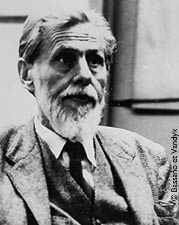
一九四九年加拿大心理學家唐納德‧赫布 Donald Hebb ── 被譽為神經心理學與神經網絡之父 ── 寫了一本
《The Organization of Behavior》
大作,提出了『學習』之『神經基礎』,今稱之為『赫布假定』 Hebb’s postulate 。這個『赫布理論』維基百科詞條這麼說︰
Hebbian theory
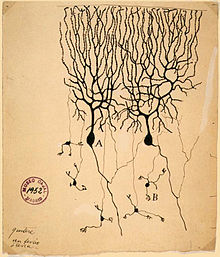
Hebbian theory is a theory in neuroscience that proposes an explanation for the adaptation of neurons in the brain during the learning process. It describes a basic mechanism for synaptic plasticity, where an increase in synaptic efficacy arises from the presynaptic cell’s repeated and persistent stimulation of the postsynaptic cell. Introduced by Donald Hebb in his 1949 book The Organization of Behavior,[1] the theory is also called Hebb’s rule, Hebb’s postulate, and cell assembly theory. Hebb states it as follows:
Let us assume that the persistence or repetition of a reverberatory activity (or “trace”) tends to induce lasting cellular changes that add to its stability.… When an axon of cell A is near enough to excite a cell B and repeatedly or persistently takes part in firing it, some growth process or metabolic change takes place in one or both cells such that A‘s efficiency, as one of the cells firing B, is increased.[1]
The theory is often summarized by Siegrid Löwel’s phrase: “Cells that fire together, wire together.” [2] However, this summary should not be taken literally. Hebb emphasized that cell A needs to “take part in firing” cell B, and such causality can only occur if cell A fires just before, not at the same time as, cell B. This important aspect of causation in Hebb’s work foreshadowed what is now known about spike-timing-dependent plasticity, which requires temporal precedence.[3] The theory attempts to explain associative or Hebbian learning, in which simultaneous activation of cells leads to pronounced increases in synaptic strength between those cells, and provides a biological basis for errorless learning methods for education and memory rehabilitation.
……
Principles
From the point of view of artificial neurons and artificial neural networks, Hebb’s principle can be described as a method of determining how to alter the weights between model neurons. The weight between two neurons increases if the two neurons activate simultaneously, and reduces if they activate separately. Nodes that tend to be either both positive or both negative at the same time have strong positive weights, while those that tend to be opposite have strong negative weights.
The following is a formulaic description of Hebbian learning: (note that many other descriptions are possible)

where  is the weight of the connection from neuron
  to neuron
  and
and  the input for neuron . Note that this is pattern learning (weights updated after every training example). In a Hopfield network, connections are set to zero if
  (no reflexive connections allowed). With binary neurons (activations either 0 or 1), connections would be set to 1 if the connected neurons have the same activation for a pattern.
Another formulaic description is:

where is the weight of the connection from neuron to neuron ,  is the number of training patterns, and
  the
the  th input for neuron . This is learning by epoch (weights updated after all the training examples are presented). Again, in a Hopfield network, connections are set to zero if (no reflexive connections).
A variation of Hebbian learning that takes into account phenomena such as blocking and many other neural learning phenomena is the mathematical model of Harry Klopf.[citation needed] Klopf’s model reproduces a great many biological phenomena, and is also simple to implement.
Generalization and stability
Hebb’s Rule is often generalized as

or the change in the th synaptic weight  is equal to a learning rate
  times the th input times the postsynaptic response
  . Often cited is the case of a linear neuron,

and the previous section’s simplification takes both the learning rate and the input weights to be 1. This version of the rule is clearly unstable, as in any network with a dominant signal the synaptic weights will increase or decrease exponentially. However, it can be shown that for any neuron model, Hebb’s rule is unstable.[5] Therefore, network models of neurons usually employ other learning theories such as BCM theory, Oja’s rule,[6] or the Generalized Hebbian Algorithm.
───
如果『赫布規則』可以證明是『unstable』不穩定,那麼重提它有什麼意義嗎?或許意義在於這是『開創者』經常遭遇的『狀況』,而『後繼者』往往可因增補而受益。故而提及於此,使得讀者可以比較其與
《W!o+ 的《小伶鼬工坊演義》︰神經網絡【Perceptron】二》
文本裡之『感知器』的『學習規則』之異同︰
The Perceptron
The next major advance was the perceptron, introduced by Frank Rosenblatt in his 1958 paper. The perceptron had the following differences from the McCullough-Pitts neuron:
- The weights and thresholds were not all identical.
- Weights can be positive or negative.
- There is no absolute inhibitory synapse.
- Although the neurons were still two-state, the output function f(u) goes from [-1,1], not [0,1]. (This is no big deal, as a suitable change in the threshold lets you transform from one convention to the other.)
- Most importantly, there was a learning rule.
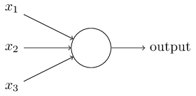
Describing this in a slightly more modern and conventional notation (and with Vi = [0,1]) we could describe the perceptron like this:

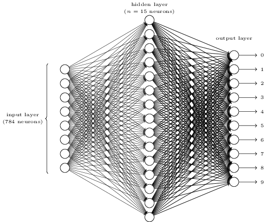
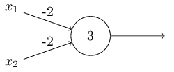
This shows a perceptron unit, i, receiving various inputs Ij, weighted by a “synaptic weight” Wij.
The ith perceptron receives its input from n input units, which do nothing but pass on the input from the outside world. The output of the perceptron is a step function:
![]()
and
![]()
For the input units, Vj = Ij. There are various ways of implementing the threshold, or bias, thetai. Sometimes it is subtracted, instead of added to the input u, and sometimes it is included in the definition of f(u).
A network of two perceptrons with three inputs would look like:

Note that they don’t interact with each other – they receive inputs only from the outside. We call this a “single layer perceptron network” because the input units don’t really count. They exist just to provide an output that is equal to the external input to the net.
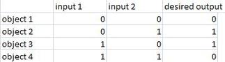
The learning scheme is very simple. Let ti be the desired “target” output for a given input pattern, and Vi be the actual output. The error (called “delta”) is the difference between the desired and the actual output, and the change in the weight is chosen to be proportional to delta.
Specifically, ![]() and
and ![]()
where ![]() is the learning rate.
is the learning rate.
Can you see why this is reasonable? Note that if the output of the ith neuron is too small, the weights of all its inputs are changed to increase its total input. Likewise, if the output is too large, the weights are changed to decrease the total input. We’ll better understand the details of why this works when we take up back propagation. First, an example.
……
如是看來『關鍵差異』就落在 ![]() 表達式的了??過去已『學會』的
表達式的了??過去已『學會』的  應該『保持』原態;尚未能『學會』的需要『將來』得減少『誤差』的吧!!
若問什麼阻礙『新觀念』 的理解?什麼導致『詮釋』的誤解??又有什麼造成用『不同概念』來『表達』的困難???誠難以回答也 !或許『學會了』意味『概念』之牢固!!曾經多次『重複』訴說很難被『改變』之耶!!!
只能邀請讀者看看與想想之前文本
如果有一個人依照波利亞 Pólya 的思考方法去『了解問題』,
【問題】
有一個農民到集市買了一隻狐狸、一隻鵝和一袋豆子,回家時要渡過一條河。河中有一條船,但是只能裝一樣東西。而且,如果沒有人看管,狐狸會吃掉鵝,而鵝又很喜歡吃豆子。問:怎樣才能讓這些東西都安全過河?
甚至這個人還能將此問題作語文的翻譯︰
《 Fox, goose and bag of beans puzzle 》
Once upon a time a farmer went to market and purchased a fox, a goose, and a bag of beans. On his way home, the farmer came to the bank of a river and rented a boat. But in crossing the river by boat, the farmer could carry only himself and a single one of his purchases – the fox, the goose, or the bag of beans.
If left together, the fox would eat the goose, or the goose would eat the beans.
The farmer’s challenge was to carry himself and his purchases to the far bank of the river, leaving each purchase intact. How did he do it?
假使有人問此人如何求解這個問題,他還能毫不猶豫的說出答案與推導過程︰
【解答】
第一步、帶鵝過河;
第二步、空手回來;
第三步、帶狐狸〔或豆子〕過河;
第四步、帶鵝回來;
第五步、帶豆子〔或狐狸〕過河;
第六步、空手回來;
第七步、帶鵝過河。
然而他也許未必可以用 pyDatalog 語言來作『表達』!這卻又是『為什麼』的呢?難道說,波利亞的方法不管用,或是我們並不『明白』它的用法,還是我們尚且不『了解』 pyDatalog 語言,以至於無法『思考』那個『表達』之法的哩??
如果此時我們想想那位『塞萬提斯』用長篇小說來『反騎士』,卻被『讀』成了擁有『阿 Q 精神』的『夢幻騎士』,也許該讚揚那些為『受壓迫』者發聲之人吧!或許須細思『非理性』和『不理性』概念之差別的吖!!
……
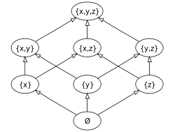
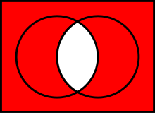
,你將會發現這個無形的『字詞網絡』框住了人們的『思維』,此正所以換個『概念體系』常常會覺得寸步難行的吧?!故而所謂的『改寫重述』多半得是『跳脫框架』的『創造性』活動。最後就讓我們歸結到俗話所講︰一圖勝千言的耶!?
【邏輯網】
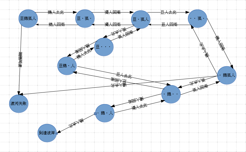
───摘自《勇闖新世界︰ 《 pyDatalog 》 導引《十》豆鵝狐人之改寫篇》
之所以言難盡意乎???

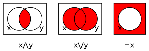
 真值表定義
真值表定義 ]
]
 ]
]
 ]
]
 ]
]

 卻矛盾!!
卻矛盾!!


 ,此處
,此處 是一個有限非空的『狀態』 state 集合
 是一個有限非空的『磁帶上字母符號』集合
 是一個『空白符號』,唯一允許在任意計算步驟中無限次出現在磁帶上的符號
 是不包含空白符號的『輸入符號』集合
 是『初始狀態』
 是『最終狀態』或稱作『接受狀態』,一般可能有
 是稱作『轉移函式』transition function,其中
  代表『讀寫頭』之向『左,右』移動,還有的增加了『不移動』no shift 的擴張
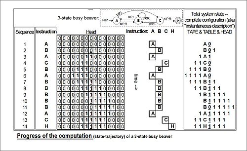

 將以下面方式運行:
 依序的從左到右填寫在磁帶之第
  編號的格子上, 將所有其它格子保持空白 ── 即填以空白符
  ──。 然後
  號格子,此時
  。 機器開始執行指令,按照轉移函式
  所描述的規則進行逐步計算。 比方如果當前機器的狀態是
  ,讀寫頭所指的格子中的符號是
  , 假使
, 假使  , 那麼機器下一步將進入新的狀態
  , 且將讀寫頭所指的格子中的符號改寫為
  , 然後把讀寫頭向左移動一個格子。 設使在某一時刻,讀寫頭所指的是第
  , 則它立刻停機並留下磁帶上的結果字串。由於轉移函式
  可能沒有可用的轉移定義, 如果在執行中遇到這種情況,機器依設計約定也將立即
  停機。
停機。