為什麼教科書裡通常有『範例』與『習題』呢?這是從『應用』的觀點考察『概念』和『原理』掌握之好壞。它使人的大腦動起來,在經過多次的『練習』以及『思辨』後,嫻熟了那個學科。
如果把『問題』比之於『感知器網絡』的『輸入』,正確『答案』就是要學會的『輸出』,

『問題』與『答案』到底哪一個比較重要呢?『撞扣之鐘』鳴有大小,本很自然之理,然而『科技』有答案的事,也許卻『人世』有問題??
《一道怪題??》已然過去,《怎樣解題》早是歷史!網路上有篇文章講︰《以色列教育部長皮隆 談盛產諾貝爾獎祕訣》
從問題中學習,思考的過程比答案更重要。又有傳聞說矽谷工程師瘋吃『聰明藥』!!作者不知 CPU 超頻、加大快捷記憶體與硬碟,果真能產生『智慧』的耶!?
── 摘自《Physical computing ︰《四》 Serial Port ︰ 3. 攔截竄訊 ‧下》
經由大量的『問題』、『答案』的『輸入』,透過減少『答案』與此刻『回答』差距之計算,逐步訓練『感知器網絡』。
解題之先,或許應多想想『解題之法』︰
《 ![]() 》網的本義就是『結網捕魚』,如今我們已經討論過多種『網』,它們雖然名稱不同,許多性質卻是一樣的。為了避免有『漏網之魚』,在此特補之以
》網的本義就是『結網捕魚』,如今我們已經討論過多種『網』,它們雖然名稱不同,許多性質卻是一樣的。為了避免有『漏網之魚』,在此特補之以
《物理哲學·中中》之文摘︰
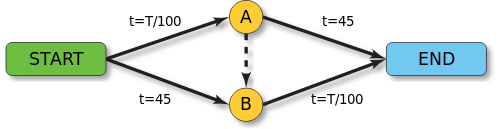
『理所當然』未必一定是『理有必然』,就像說『改善交通』應該『多開條路』的吧!!德國數學家迪特里希‧布雷斯 Dietrich Braess 宣稱︰
在一個交通網上新闢一條通路,反而可能使得用路所需的時間增加了;這一條新闢的道路,非但無助於減少交通遲滯,卻很可能會降低了整個交通網的服務水準。


納什均衡, 

如果  ,最佳選擇
,最佳選擇


……
那麼一個人要 是『開通思路』,他是否『推理』會變得更慢的呢?也許『豆鵝狐人』的回答是︰人類的『思維』一般會形成『定勢』 ,因此通常只見着『陽關道』,少會過『獨木橋』,故而很難發生布雷斯的悖論,還是『思多識廣』的好吧!但是告誡勇闖新世界的人們,小心所創作的『人工智 慧』機器,最好不要一不小心,它卻變成『傻鳥』的了??
這樣說來喬治‧波利亞的『怎樣解題』之法

喬治‧波利亞
George Pólya
suggests the following steps when solving a mathematical problem:
1. First, you have to understand the problem.
2. After understanding, then make a plan.
3. Carry out the plan.
4. Look back on your work. How could it be better?
If this technique fails, Pólya advises: “If you can’t solve a problem, then there is an easier problem you can solve: find it.” Or: “If you cannot solve the proposed problem, try to solve first some related problem. Could you imagine a more accessible related problem?”
喬治‧波利亞長期從事數學教學,對數學思維的一般規律有深入的研究,一生推動數學教育。一九五四年,波利亞寫了兩卷不同於一般的數學書《Induction And_Analogy In Mathematics》與《Patterns Of Plausible Inference》探討『啟發式』之『思維樣態』,這常常是一種《數學發現》之切入點,也是探尋『常識徵候』中的『合理性』根源。舉個例子來說,典型的亞里斯多德式的『三段論』 syllogisms ︰

 真,
真,  真。
真。
如果對比著『似合理的』Plausible 『推理』︰
 真, 更可能是真。
這種『推理』一般稱之為『肯定後件』 的『邏輯誤謬』。因為在『邏輯』上,這種『形式』的推導,並不『必然的』保障『歸結』一定是『真』的。然而這種『推理形式』是完全沒有『道理』的嗎?如果從『三段論』之『邏輯』上來講,要是 為『假』, 也就『必然的』為『假』。所以假使 為『真』之『必要條件』 為『真』,那麼 不該是『更可能』是『真』的嗎??
,一點不因提出時間古早,依然是管用的!若說應用之妙在於『能想人所不能想』和『能用人所不能用』,此法終究使人困惑?然而一個『困思勉行』者時有感悟,一位『真積力』者,己不能通,神自來通,又何困惑之有的呢!!
─── 摘自《勇闖新世界︰ 《 pyDatalog 》 導引《十》豆鵝狐人之推理篇》
複習重要的『概念』︰
Perceptron
Definition
In the modern sense, the perceptron is an algorithm for learning a binary classifier: a function that maps its input  (a real-valued vector) to an output value
  (a single binary value):
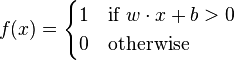
where w is a vector of real-valued weights,  is the dot product
  , where m is the number of inputs to the perceptron and b is the bias. The bias shifts the decision boundary away from the origin and does not depend on any input value.
The value of (0 or 1) is used to classify x as either a positive or a negative instance, in the case of a binary classification problem. If  is negative, then the weighted combination of inputs must produce a positive value greater than
  in order to push the classifier neuron over the 0 threshold. Spatially, the bias alters the position (though not the orientation) of the decision boundary. The perceptron learning algorithm does not terminate if the learning set is not linearly separable. If the vectors are not linearly separable learning will never reach a point where all vectors are classified properly. The most famous example of the perceptron’s inability to solve problems with linearly nonseparable vectors is the Boolean exclusive-or problem. The solution spaces of decision boundaries for all binary functions and learning behaviors are studied in the reference.[7]
In the context of neural networks, a perceptron is an artificial neuron using the Heaviside step function as the activation function. The perceptron algorithm is also termed the single-layer perceptron, to distinguish it from a multilayer perceptron, which is a misnomer for a more complicated neural network. As a linear classifier, the single-layer perceptron is the simplest feedforward neural network.
Learning algorithm
Below is an example of a learning algorithm for a (single-layer) perceptron. For multilayer perceptrons, where a hidden layer exists, more sophisticated algorithms such as backpropagation must be used. Alternatively, methods such as the delta rule can be used if the function is non-linear and differentiable, although the one below will work as well.
When multiple perceptrons are combined in an artificial neural network, each output neuron operates independently of all the others; thus, learning each output can be considered in isolation.
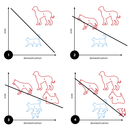
A diagram showing a perceptron updating its linear boundary as more training examples are added.
Definitions
We first define some variables:
 denotes the output from the perceptron for an input vector
  .
. is the training set of
  samples, where:
 is the
  -dimensional input vector.
 is the desired output value of the perceptron for that input.
We show the values of the features as follows:
 is the value of the
  th feature of the
  th training input vector.
 .
.
To represent the weights:
 is the th value in the weight vector, to be multiplied by the value of the th input feature.
- Because , the
 is effectively a learned bias that we use instead of the bias constant .
To show the time-dependence of  , we use:
 is the weight at time
  .
. is the learning rate, where
  .
.
Too high a learning rate makes the perceptron periodically oscillate around the solution unless additional steps are taken.
Steps
- Initialize the weights and the threshold. Weights may be initialized to 0 or to a small random value. In the example below, we use 0.
- For each example j in our training set D, perform the following steps over the input
 and desired output :
- Calculate the actual output:
- Update the weights:
 , for all features
  .
.
- Calculate the actual output:
- For offline learning, the step 2 may be repeated until the iteration error
 is less than a user-specified error threshold
  , or a predetermined number of iterations have been completed.

The algorithm updates the weights after steps 2a and 2b. These weights are immediately applied to a pair in the training set, and subsequently updated, rather than waiting until all pairs in the training set have undergone these steps.
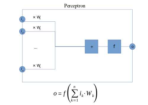
The appropriate weights are applied to the inputs, and the resulting weighted sum passed to a function that produces the output o.
然後提槍上陣耶︰
Example
A perceptron learns to perform a binary NAND function on inputs  and
and  .
.
- Inputs:
 , , , with input held constant at 1.
 - Threshold (): 0.5
- Bias (): 1
- Learning rate (
 ): 0.1
 - Training set, consisting of four samples:

In the following, the final weights of one iteration become the initial weights of the next. Each cycle over all the samples in the training set is demarcated with heavy lines.
……
This example can be implemented in the following Python code.
threshold = 0.5
learning_rate = 0.1
weights = [0, 0, 0]
training_set = [((1, 0, 0), 1), ((1, 0, 1), 1), ((1, 1, 0), 1), ((1, 1, 1), 0)]

def dot_product(values, weights):
    return sum(value * weight for value, weight in zip(values, weights))

while True:
    print('-' * 60)
    error_count = 0
    for input_vector, desired_output in training_set:
        print(weights)
        result = dot_product(input_vector, weights) > threshold
        error = desired_output - result
        if error != 0:
            error_count += 1
            for index, value in enumerate(input_vector):
                weights[index] += learning_rate * error * value
    if error_count == 0:
        break