即使在工程力學

Applied mechanics

Applied mechanics (also engineering mechanics) is a branch of the physical sciences and the practical application of mechanics. Pure mechanics describes the response of bodies (solids and fluids) or systems of bodies to external forces. Some examples of mechanical systems include the flow of a liquid under pressure, the fracture of a solid from an applied force, or the vibration of an ear in response to sound. A practitioner of the discipline is known as a mechanician.

Applied mechanics describes the behavior of a body, in either a beginning state of rest or of motion, subjected to the action of forces.^[1] Applied mechanics, bridges the gap between physical theory and its application totechnology. It is used in many fields of engineering, especially mechanical engineering and civil engineering. In this context, it is commonly referred to as Engineering Mechanics. Much of modern engineering mechanics is based on Isaac Newton‘s laws of motion while the modern practice of their application can be traced back to Stephen Timoshenko, who is said to be the father of modern engineering mechanics.

Within the practical sciences, applied mechanics is useful in formulating new ideas and theories, discovering and interpreting phenomena, and developing experimental and computational tools. In the application of thenatural sciences, mechanics was said to be complemented by thermodynamics, the study of heat and more generally energy, and electromechanics, the study of electricity and magnetism.^[2]

的領域中，拉格朗日力學容易使用廣義座標，故有其優異之處︰

From Newtonian to Lagrangian mechanics

Newton’s laws

For simplicity, Newton’s laws can be illustrated for one particle without much loss of generality (for a system of N particles, all of these equations apply to each particle in the system). The equation of motion for particle of mass m is Newton’s second law of 1687, in modern vector notation

$\displaystyle \mathbf {F} =m\mathbf {a} \,,$

where a is its acceleration and F the resultant force acting on it. In three spatial dimensions, this is a system of three coupled second order ordinary differential equations to solve, since there are three components in this vector equation. The solutions are the position vectors r of the particles at time t, subject to the initial conditions of r and v when t = 0.

Newton’s laws are easy to use in Cartesian coordinates, but Cartesian coordinates are not always convenient, and for other coordinate systems the equations of motion can become complicated. In a set of curvilinear coordinates ξ = (ξ¹, ξ²,ξ³), the law in tensor index notation is the “Lagrangian form”^[15]^[16]

$\displaystyle F^{a}=m\left({\frac {\mathrm {d} ^{2}\xi ^{a}}{\mathrm {d} t^{2}}}+\Gamma ^{a}{}_{bc}{\frac {\mathrm {d} \xi ^{b}}{\mathrm {d} t}}{\frac {\mathrm {d} \xi ^{c}}{\mathrm {d} t}}\right)={\frac {\mathrm {d} }{\mathrm {d} t}}{\frac {\partial T}{\partial {\dot {\xi }}^{a}}}-{\frac {\partial T}{\partial \xi ^{a}}}\,,\quad {\dot {\xi }}^{a}\equiv {\frac {\mathrm {d} \xi ^{a}}{\mathrm {d} t}}\,,$

where F^a is the ath contravariant components of the resultant force acting on the particle, Γ^a_bc are the Christoffel symbols of the second kind,

$\displaystyle T={\frac {1}{2}}mg_{bc}{\frac {\mathrm {d} \xi ^{b}}{\mathrm {d} t}}{\frac {\mathrm {d} \xi ^{c}}{\mathrm {d} t}}\,,$

is the kinetic energy of the particle, and g_bc the covariant components of the metric tensor of the curvilinear coordinate system. All the indices a, b, c, each take the values 1, 2, 3. Curvilinear coordinates are not the same as generalized coordinates.

It may seem like an overcomplication to cast Newton’s law in this form, but there are advantages. The acceleration components in terms of the Christoffel symbols can be avoided by evaluating derivatives of the kinetic energy instead. If there is no resultant force acting on the particle, F = 0, it does not accelerate, but moves with constant velocity in a straight line. Mathematically, the solutions of the differential equation are geodesics, the curves of extremal length between two points in space (These may end up being minimal so the shortest paths, but that is not necessary). In flat 3d real space the geodesics are simply straight lines. So for a free particle, Newton’s second law coincides with the geodesic equation, and states free particles follow geodesics, the extremal trajectories it can move along. If the particle is subject to forces, F ≠ 0, the particle accelerates due to forces acting on it, and deviates away from the geodesics it would follow if free. With appropriate extensions of the quantities given here in flat 3d space to 4d curved spacetime, the above form of Newton’s law also carries over to Einstein‘s general relativity, in which case free particles follow geodesics in curved spacetime that are no longer “straight lines” in the ordinary sense.^[17]

However, we still need to know the total resultant force F acting on the particle, which in turn requires the resultant non-constraint force N plus the resultant constraint force C,

$\displaystyle \mathbf {F} =\mathbf {C} +\mathbf {N} \,.$

The constraint forces can be complicated, since they will generally depend on time. Also, if there are constraints, the curvilinear coordinates are not independent but related by one or more constraint equations.

The constraint forces can either be eliminated from the equations of motion so only the non-constraint forces remain, or included by including the constraint equations in the equations of motion.

如果再乘著

D’Alembert’s principle

A fundamental result in analytical mechanics is D’Alembert’s principle, introduced in 1708 by Jacques Bernoulli to understand static equilibrium, and developed by D’Alembert in 1743 to solve dynamical problems.^[18] The principle asserts for N particles^[10]

$\displaystyle \sum _{k=1}^{N}(\mathbf {N} _{k}+\mathbf {C} _{k}-m_{k}\mathbf {a} _{k})\cdot \delta \mathbf {r} _{k}=0\,.$

The δr_k are virtual displacements, by definition they are infinitesimal changes in the configuration of the system consistent with the constraint forces acting on the system at an instant of time,^[19] i.e. in such a way that the constraint forces maintain the constrained motion. They are not the same as the actual displacements in the system, which are caused by the resultant constraint and non-constraint forces acting on the particle to accelerate and move it.^{[nb 2]} Virtual work is the work done along a virtual displacement for any force (constraint or non-constraint).

Since the constraint forces act perpendicular to the motion of each particle in the system to maintain the constraints, the total virtual work by the constraint forces acting on the system is zero;^[20]^{[nb 3]}

$\displaystyle \sum _{k=1}^{N}\mathbf {C} _{k}\cdot \delta \mathbf {r} _{k}=0\,,$

so that

$\displaystyle \sum _{k=1}^{N}(\mathbf {N} _{k}-m_{k}\mathbf {a} _{k})\cdot \delta \mathbf {r} _{k}=0\,.$

Thus D’Alembert’s principle allows us to concentrate on only the applied non-constraint forces, and exclude the constraint forces in the equations of motion.^[21]^[22] The form shown is also independent of the choice of coordinates. However, it cannot be readily used to set up the equations of motion in an arbitrary coordinate system since the displacements δr_k might be connected by a constraint equation, which prevents us from setting the N individual summands to 0. We will therefore seek a system of mutually independent coordinates for which the total sum will be 0 if and only if the individual summands are 0. Setting each of the summands to 0 will eventually give us our separated equations of motion.

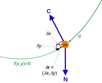
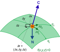
One degree of freedom. Two degrees of freedom.

Constraint force C and virtual displacement δr for a particle of mass mconfined to a curve. The resultant non-constraint force is N.

之羽翼，利於跨越

約束 (經典力學)

在經典力學裏，物體的運動必須遵守牛頓運動定律。除此以外，每一個物理系統時常會有一些約束，物體的運動也必須遵守這些約束。例如，簡單擺系統的約束是擺繩的長度是常數，擺錘與支撐點的距離必須是這長度。除非水瓶破了，一個封閉的水瓶裏的水分子，絕對不能運動到水瓶的外面。這些約束使物理系統的特性呈現出來。要分析一個物理系統，必須了解這系統裏的約束。

因為約束的作用，在分析物體的運動上，會遇到一些新的困難：

許多描述物體運動的位置不再互相獨立。如果這約束是完整約束，可以用廣義坐標來除去一些相關的位置。如果整個系統是完整系統，可以用獨立的廣義坐標來表示這個系統的運動。通常，可以找到相關的形式論來分析這個系統的運動。
假若一個物體的運動因為約束而改變，則必定有一個關於這約束的力作用於這物體上；不然，這物體的運動不會改變。稱此力為約束力。一般而言，事先並不知道約束力的值量。如果能將一個系統所有的廣義坐標都轉換成互不相關的廣義坐標，那麼，不需要知道約束力，就可以求得物體的運動方程式了^[1]。

的門檻，直指運動方程式也！

Equations of motion from D’Alembert’s principle

If there are constraints on particle k, then since the coordinates of the position r_k = (x_k, y_k, z_k) are linked together by a constraint equation, so are those of the virtual displacements δr_k = (δx_k, δy_k,δz_k). Since the generalized coordinates are independent, we can avoid the complications with the δr_k by converting to virtual displacements in the generalized coordinates. These are related in the same form as a total differential,^[23]

$\displaystyle \delta \mathbf {r} _{k}=\sum _{j=1}^{n}{\frac {\partial \mathbf {r} _{k}}{\partial q_{j}}}\delta q_{j}\,.$

There is no partial time derivative with respect to time multiplied by a time increment, since this is a virtual displacement, one along the constraints in an instant of time.

The first term in D’Alembert’s principle above is the virtual work done by the non-constraint forces N_k along the virtual displacements δr_k, and can without loss of generality be converted into the generalized analogues by the definition of generalized forces

$\displaystyle Q_{j}=\sum _{k=1}^{N}\mathbf {N} _{k}\cdot {\frac {\partial \mathbf {r} _{k}}{\partial q_{j}}}\,,$

so that

$\displaystyle \sum _{k=1}^{N}\mathbf {N} _{k}\cdot \delta \mathbf {r} _{k}=\sum _{k=1}^{N}\mathbf {N} _{k}\cdot \sum _{j=1}^{n}{\frac {\partial \mathbf {r} _{k}}{\partial q_{j}}}\delta q_{j}=\sum _{j=1}^{n}Q_{j}\delta q_{j}\,.$

This is half of the conversion to generalized coordinates. It remains to convert the acceleration term into generalized coordinates, which is not immediately obvious. Recalling the Lagrange form of Newton’s second law, the partial derivatives of the kinetic energy with respect to the generalized coordinates and velocities can be found to give the desired result;^[24]

$\displaystyle \sum _{k=1}^{N}m_{k}\mathbf {a} _{k}\cdot {\frac {\partial \mathbf {r} _{k}}{\partial q_{j}}}={\frac {\mathrm {d} }{\mathrm {d} t}}{\frac {\partial T}{\partial {\dot {q}}_{j}}}-{\frac {\partial T}{\partial q_{j}}}\,.$

Now D’Alembert’s principle is in the generalized coordinates as required,

$\displaystyle \sum _{j=1}^{n}\left[Q_{j}-\left({\frac {\mathrm {d} }{\mathrm {d} t}}{\frac {\partial T}{\partial {\dot {q}}_{j}}}-{\frac {\partial T}{\partial q_{j}}}\right)\right]\delta q_{j}=0\,,$

and since these virtual displacements δq_j are independent and nonzero, the coefficients can be equated to zero, resulting in Lagrange’s equations^[25]^[26] or the generalized equations of motion,^[27]

$\displaystyle Q_{j}={\frac {\mathrm {d} }{\mathrm {d} t}}{\frac {\partial T}{\partial {\dot {q}}_{j}}}-{\frac {\partial T}{\partial q_{j}}}$

These equations are equivalent to Newton’s laws for the non-constraint forces. The generalized forces in this equation are derived from the non-constraint forces only – the constraint forces have been excluded from D’Alembert’s principle and do not need to be found. The generalized forces may be non-conservative, provided they satisfy D’Alembert’s principle.^[28]

且借例釋以明之呦☆

Simple pendulum

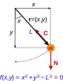
Simple pendulum. Since the rod is rigid, the position of the bob is constrained according to the equation f(x, y) = 0, the constraint force C is the tension in the rod. Again the non-constraint force Nin this case is gravity.

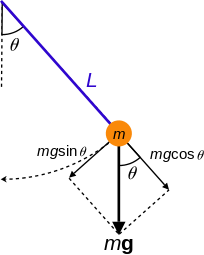
Dynamic model of a simple pendulum.

The relationship between the use of generalized coordinates and Cartesian coordinates to characterize the movement of a mechanical system can be illustrated by considering the constrained dynamics of a simple pendulum.^[12]^[13]

A simple pendulum consists of a mass M hanging from a pivot point so that it is constrained to move on a circle of radius L. The position of the mass is defined by the coordinate vector r=(x, y) measured in the plane of the circle such that y is in the vertical direction. The coordinates x and y are related by the equation of the circle

$\displaystyle f(x,y)=x^{2}+y^{2}-L^{2}=0,$

that constrains the movement of M. This equation also provides a constraint on the velocity components,

$\displaystyle {\dot {f}}(x,y)=2x{\dot {x}}+2y{\dot {y}}=0.$

Now introduce the parameter θ, that defines the angular position of M from the vertical direction. It can be used to define the coordinates x and y, such that

$\displaystyle \mathbf {r} =(x,y)=(L\sin \theta ,-L\cos \theta ).$

The use of θ to define the configuration of this system avoids the constraint provided by the equation of the circle.

Notice that the force of gravity acting on the mass m is formulated in the usual Cartesian coordinates,

$\displaystyle \mathbf {F} =(0,-mg),$

where g is the acceleration of gravity.

The virtual work of gravity on the mass m as it follows the trajectory r is given by

$\displaystyle \delta W=\mathbf {F} \cdot \delta \mathbf {r} .$

The variation δr can be computed in terms of the coordinates x and y, or in terms of the parameter θ,

$\displaystyle \delta \mathbf {r} =(\delta x,\delta y)=(L\cos \theta ,L\sin \theta )\delta \theta .$

Thus, the virtual work is given by

$\displaystyle \delta W=-mg\delta y=-mgL\sin \theta \delta \theta .$

Notice that the coefficient of δy is the y-component of the applied force. In the same way, the coefficient of δθ is known as the generalized force along generalized coordinate θ, given by

$\displaystyle F_{\theta }=-mgL\sin \theta .$

To complete the analysis consider the kinetic energy T of the mass, using the velocity,

$\displaystyle \mathbf {v} =({\dot {x}},{\dot {y}})=(L\cos \theta ,L\sin \theta ){\dot {\theta }},$

so,

$\displaystyle T={\frac {1}{2}}m\mathbf {v} \cdot \mathbf {v} ={\frac {1}{2}}m({\dot {x}}^{2}+{\dot {y}}^{2})={\frac {1}{2}}mL^{2}{\dot {\theta }}^{2}.$

D’Alembert’s form of the principle of virtual work for the pendulum in terms of the coordinates x and y are given by,

$\displaystyle {\frac {d}{dt}}{\frac {\partial T}{\partial {\dot {x}}}}-{\frac {\partial T}{\partial x}}=F_{x}+\lambda {\frac {\partial f}{\partial x}},\quad {\frac {d}{dt}}{\frac {\partial T}{\partial {\dot {y}}}}-{\frac {\partial T}{\partial y}}=F_{y}+\lambda {\frac {\partial f}{\partial y}}.$

This yields the three equations

$\displaystyle m{\ddot {x}}=\lambda (2x),\quad m{\ddot {y}}=-mg+\lambda (2y),\quad x^{2}+y^{2}-L^{2}=0,$

in the three unknowns, x, y and λ.

Using the parameter θ, those equations take the form

$\displaystyle {\frac {d}{dt}}{\frac {\partial T}{\partial {\dot {\theta }}}}-{\frac {\partial T}{\partial \theta }}=F_{\theta },$

which becomes,

$\displaystyle mL^{2}{\ddot {\theta }}=-mgL\sin \theta ,$

$\displaystyle {\ddot {\theta }}+{\frac {g}{L}}\sin \theta =0.$

This formulation yields one equation because there is a single parameter and no constraint equation.

This shows that the parameter θ is a generalized coordinate that can be used in the same way as the Cartesian coordinates x and y to analyze the pendulum.

FreeSandal

每日彙整: 2018-04-15

STEM 隨筆︰古典力學︰運動學【三‧IV 】