法國的儒勒‧昂利‧龐加萊 Jules Henri Poincaré 最偉大的數學家之一,理論科學家和科學哲學家。他被公認為是十九世紀末與二十世紀初的數學領袖,一位繼天才高斯之後對數學及其應用具有全面知識之最後一人。他在數學、物理數學和天體力學上都有很多獨創性的貢獻。龐加萊提出的『龐加萊猜想』是數學中最著名的問題之一 ,一個克雷數學研究所所懸賞求解的七大千禧年數學難題 ──,二零零六年確認由俄羅斯數學家格里戈里‧佩雷爾曼 ригорий Яковлевич Перельман 完成最終證明,亦在同年獲得菲爾茲獎,但他卻並未現身領獎 ── 。龐加萊在物理學『三體問題』之研究中的發現,使他成了知道『確定性系統』之『混沌』現象的第一人,並為今天的『混沌理論』打下了基礎。
一個質量  物體,初始位置在
  ,初始速度為
  ,在
,在  軸上運動,依據牛頓的第二運動定律,它的運動滿足一個二階微分方程式︰

一般而言,除了一些特殊的力  的形式,比方說簡諧運動之線性彈力
  ,微分方程式很難有『確解』,大概都得用『數值分析』的方式求解。那麼有沒有另一種運動描述辦法的呢?龐加萊和玻爾茲曼 Boltzmann 等人發展了『相空間』phase space 的想法,因為物體一旦給定了初始位置與初始速度── 一般使用動量
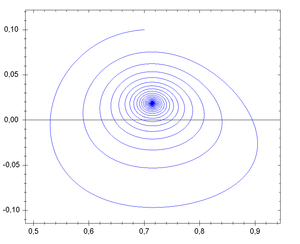
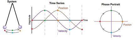
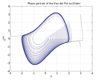
  ──,它的運動軌跡就由牛頓的第二運動定律所確定,相空間是一個 (位置,動量) 所構成的座標系,這樣該物體的運動軌跡就畫出了相空間裡的一條線 ── 叫做相圖 phase diagram ──。一般這條曲線不會『自相交』,因為相交代表有不同的運動軌跡可以選擇,所以一旦相交會就只能是一種『週期運動』。龐加萊在研究三體問題的相圖時,卻發現只要『初始點』── 位置或動量 ──,極微小的變化,相圖就發生很大的改變,這種『敏感性』可能導致系統的『不可預測性』或是『不穩定性』。那我們的太陽系是穩定的嗎??
現今的混沌理論 Chaos theory 描述『非線性』系統在一定參數條件下會發生『分岔』 bifurcation 現象,周期運動與非周期運動可能相互『糾纏』,以至於通往某種非周期又可以有序之運動理論 。因此它是一種兼具『定性』與『定量』的分析之思考方法,用以探討動力系統中無法僅用『一時單一』的數據,必須用『連續整體』的數據才能加以解釋或是描述該系統之行為。

『混沌』chaos 一詞源自古希臘哲學家認為宇宙起源於混亂無序的狀態,逐漸由這個混沌之初形成現今有條不紊的世界。這個混沌論說︰
一切事物的初始狀態,都只是一些看似無關的碎片,然而當此混沌過程結束之時,這些碎片終自主有序的聚合成一個整體。
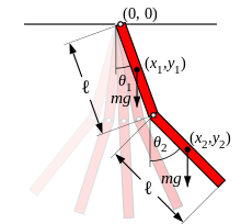
左圖演示一個『雙擺』Double pendulum 的運動,系統總能量取某些數量時它的運動是混沌的。假使想要對它『數值』求解 ,從『數值分析』的程式設計觀點來看這個數據『敏感性』問題 ── 叫做『惡劣條件』ill condition ──,通常需要作多次多種『收斂測試』,否則到底計算出來的是什麼,可就說不清的了。有興趣物理、數學或寫程式的讀者可以參考︰
─── 《混沌理論》
假使將牛頓運動方程式表述為

 。
。
因是  構成了相空間,設當時間
  時,此系統處於
  狀態,正言『初值問題』也︰
Initial value problem
In mathematics, the field of differential equations, an initial value problem (also called the Cauchy problem by some authors) is an ordinary differential equation together with a specified value, called the initial condition, of the unknown function at a given point in the domain of the solution. In physics or other sciences, modeling a system frequently amounts to solving an initial value problem; in this context, the differential initial value is an equation that is an evolution equation specifying how, given initial conditions, the system will evolve with time.
Definition
An initial value problem is a differential equation
 with
with  where
where  is an open set of
  ,
,
together with a point in the domain of
 ,
,
called the initial condition.
A solution to an initial value problem is a function  that is a solution to the differential equation and satisfies
 .
.
In higher dimensions, the differential equation is replaced with a family of equations  , and
, and  is viewed as the vector
  . More generally, the unknown function can take values on infinite dimensional spaces, such as Banach spaces or spaces of distributions.
Initial value problems are extended to higher orders by treating the derivatives in the same way as an independent function, e.g.  .
.
Existence and uniqueness of solutions
For a large class of initial value problems, the existence and uniqueness of a solution can be illustrated through the use of a calculator.
The Picard–Lindelöf theorem guarantees a unique solution on some interval containing t0 if ƒ is continuous on a region containing t0 and y0 and satisfies the Lipschitz condition on the variable y. The proof of this theorem proceeds by reformulating the problem as an equivalent integral equation. The integral can be considered an operator which maps one function into another, such that the solution is a fixed point of the operator. The Banach fixed point theorem is then invoked to show that there exists a unique fixed point, which is the solution of the initial value problem.
An older proof of the Picard–Lindelöf theorem constructs a sequence of functions which converge to the solution of the integral equation, and thus, the solution of the initial value problem. Such a construction is sometimes called “Picard’s method” or “the method of successive approximations”. This version is essentially a special case of the Banach fixed point theorem.
Hiroshi Okamura obtained a necessary and sufficient condition for the solution of an initial value problem to be unique. This condition has to do with the existence of a Lyapunov function for the system.
In some situations, the function ƒ is not of class C1, or even Lipschitz, so the usual result guaranteeing the local existence of a unique solution does not apply. The Peano existence theorem however proves that even for ƒ merely continuous, solutions are guaranteed to exist locally in time; the problem is that there is no guarantee of uniqueness. The result may be found in Coddington & Levinson (1955, Theorem 1.3) or Robinson (2001, Theorem 2.6). An even more general result is the Carathéodory existence theorem, which proves existence for some discontinuous functions ƒ.
此說焉能不適用於拉格朗日力學哩?!
但
Nonminimal Coordinates Pendulum
In this example we demonstrate the use of the functionality provided in mechanics for deriving the equations of motion (EOM) for a pendulum with a nonminimal set of coordinates. As the pendulum is a one degree of freedom system, it can be described using one coordinate and one speed (the pendulum angle, and the angular velocity respectively). Choosing instead to describe the system using the and  coordinates of the mass results in a need for constraints. The system is shown below:

The system will be modeled using both Kane’s and Lagrange’s methods, and the resulting EOM linearized. While this is a simple problem, it should illustrate the use of the linearization methods in the presence of constraints.
範例不及明講呦!?
‧ 拉格朗日方程式
![\left[\begin{matrix}- g m + m \frac{d^{2}}{d t^{2}} \operatorname{q_{1}}{\left (t \right )} + 2 \operatorname{lam_{1}}{\left (t \right )} \operatorname{q_{1}}{\left (t \right )}\\m \frac{d^{2}}{d t^{2}} \operatorname{q_{2}}{\left (t \right )} + 2 \operatorname{lam_{1}}{\left (t \right )} \operatorname{q_{2}}{\left (t \right )}\end{matrix}\right]](http://www.freesandal.org/wp-content/ql-cache/quicklatex.com-c72a1b5ec3a0ebc8b3a9bb6a70ebeb75_l3.png "Rendered by QuickLaTeX.com")
‧ 符號動力學系統矩陣
![\left[\begin{matrix}1 & 0 & 0 & 0 & 0\\0 & 1 & 0 & 0 & 0\\0 & 0 & m & 0 & - 2 \operatorname{q_{1}}{\left (t \right )}\\0 & 0 & 0 & m & - 2 \operatorname{q_{2}}{\left (t \right )}\\0 & 0 & 2 \operatorname{q_{1}}{\left (t \right )} & 2 \operatorname{q_{2}}{\left (t \right )} & 0\end{matrix}\right] \ \left[\begin{matrix} \dot{q_1} \\\dot{q_2}\\\ddot{q_1} \\\ddot{q_2}\\{-lam}_1 \end{matrix}\right] = \ \left[\begin{matrix}\frac{d}{d t} \operatorname{q_{1}}{\left (t \right )}\\\frac{d}{d t} \operatorname{q_{2}}{\left (t \right )}\\g m\\0\\- 2 \frac{d}{d t} \operatorname{q_{1}}{\left (t \right )}^{2} - 2 \frac{d}{d t} \operatorname{q_{2}}{\left (t \right )}^{2}\end{matrix}\right]](http://www.freesandal.org/wp-content/ql-cache/quicklatex.com-b3c2fe2d8ac8a46c3f3b795a51f0f15d_l3.png "Rendered by QuickLaTeX.com")
‧ 狀態方程式
rhs(inv_method=None, **kwargs)
Returns equations that can be solved numerically
| Parameters: |
inv_method : str
|
|---|
![\left[\begin{matrix}\frac{d}{d t} \operatorname{q_{1}}{\left (t \right )}\\\frac{d}{d t} \operatorname{q_{2}}{\left (t \right )}\\\frac{1}{m} \left(g m + \frac{2 \operatorname{q_{1}}{\left (t \right )}}{\frac{4}{m} \operatorname{q_{1}}^{2}{\left (t \right )} + \frac{4}{m} \operatorname{q_{2}}^{2}{\left (t \right )}} \left(- 2 g \operatorname{q_{1}}{\left (t \right )} - 2 \frac{d}{d t} \operatorname{q_{1}}{\left (t \right )}^{2} - 2 \frac{d}{d t} \operatorname{q_{2}}{\left (t \right )}^{2}\right)\right)\\\frac{2 \operatorname{q_{2}}{\left (t \right )}}{m \left(\frac{4}{m} \operatorname{q_{1}}^{2}{\left (t \right )} + \frac{4}{m} \operatorname{q_{2}}^{2}{\left (t \right )}\right)} \left(- 2 g \operatorname{q_{1}}{\left (t \right )} - 2 \frac{d}{d t} \operatorname{q_{1}}{\left (t \right )}^{2} - 2 \frac{d}{d t} \operatorname{q_{2}}{\left (t \right )}^{2}\right)\\\frac{1}{\frac{4}{m} \operatorname{q_{1}}^{2}{\left (t \right )} + \frac{4}{m} \operatorname{q_{2}}^{2}{\left (t \right )}} \left(- 2 g \operatorname{q_{1}}{\left (t \right )} - 2 \frac{d}{d t} \operatorname{q_{1}}{\left (t \right )}^{2} - 2 \frac{d}{d t} \operatorname{q_{2}}{\left (t \right )}^{2}\right)\end{matrix}\right]](http://www.freesandal.org/wp-content/ql-cache/quicklatex.com-c23b0840dd6fc64e949af02500bf9d2f_l3.png "Rendered by QuickLaTeX.com")