該怎麼看待有兩個部份  ,又似一個整體
  的複數呢?莫非歐拉的上帝遣之來
  ,不得不全純乎??
全純函數(holomorphic function)是複分析研究的中心對象;它們是定義在複平面C的開子集上的,在複平面C中取值的,在每點上皆複可微的函數。這是比實可微強得多的條件,暗示著此函數無窮可微並可以用泰勒級數來描述。
解析函數(analytic function)一詞經常可以和「全純函數」互相交換使用,雖然前者有幾個其他含義。
全純函數有時稱為正則函數。在整個複平面上都全純的函數稱為整函數(entire function)。「在一點a全純」不僅表示在a可微,而且表示在某個中心為a的複平面的開鄰域上可微。雙全純(biholomorphic)表示一個有全純逆函數的全純函數。
Terminology
The word “holomorphic” was introduced by two of Cauchy‘s students, Briot (1817–1882) and Bouquet (1819–1895), and derives from the Greek ὅλος (holos) meaning “entire”, and μορφή (morphē) meaning “form” or “appearance”.[9]
Today, the term “holomorphic function” is sometimes preferred to “analytic function”, as the latter is a more general concept. This is also because an important result in complex analysis is that every holomorphic function is complex analytic, a fact that does not follow directly from the definitions. The term “analytic” is however also in wide use.
故而必得條條道路皆通羅馬也耶!
……
因任意  可以看成
可以看成  的形式,可設想
  、
、 都能表示為
都能表示為  算符也。此處係數
  之定,只需援用
  之獨立性
之獨立性  、
、 ;
;  、
、 就得矣◎
就得矣◎
─── 《觀察者《變換‧D 》》
何事 JULIUS O. SMITH III 先生用一整章
談『正弦波』呢?
為什麼高舉『廣義相量』大旗呦!
因為借之可統攝多種常用變換也!?
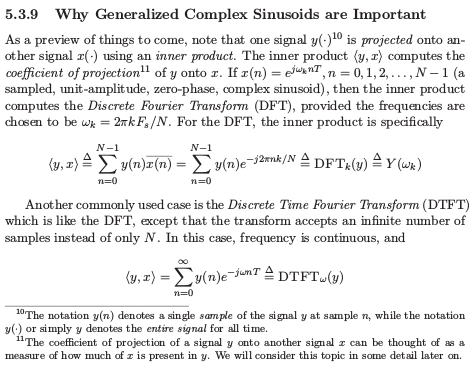
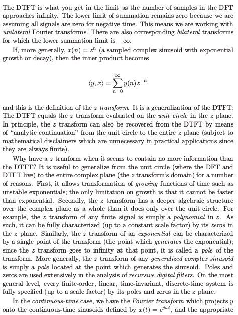
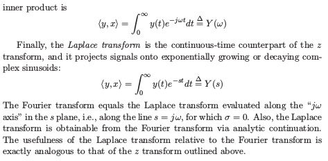
Importance of Generalized Complex Sinusoids
明白希爾伯特變換之重要性勒◎
Hilbert transform
In mathematics and in signal processing, the Hilbert transform is a linear operator that takes a function, u(t) of a real variable and produces another function of a real variable H(u)(t).
The Hilbert transform is important in signal processing, where it derives the analytic representation of a signal u(t). This means that the real signal u(t) is extended into the complex plane such that it satisfies the Cauchy–Riemann equations. For example, the Hilbert transform leads to the harmonic conjugate of a given function in Fourier analysis, aka harmonic analysis. Equivalently, it is an example of a singular integral operator and of a Fourier multiplier.
The Hilbert transform was originally defined for periodic functions, or equivalently for functions on the circle, in which case it is given by convolution with the Hilbert kernel. More commonly, however, the Hilbert transform refers to a convolution with the Cauchy kernel, for functions defined on the real lineR (the boundary of the upper half-plane). The Hilbert transform is closely related to the Paley–Wiener theorem, another result relating holomorphic functions in the upper half-plane and Fourier transforms of functions on the real line.
The Hilbert transform is named after David Hilbert, who first introduced the operator to solve a special case of the Riemann–Hilbert problem for holomorphic functions.
![]()
The Hilbert transform, in red, of a square wave, in blue
……
Hilbert transform in signal processing
Bedrosian’s theorem
Bedrosian’s theorem states that the Hilbert transform of the product of a low-pass and a high-pass signal with non-overlapping spectra is given by the product of the low-pass signal and the Hilbert transform of the high-pass signal, or

where fLP and fHP are the low- and high-pass signals respectively (Schreier & Scharf 2010, 14).
Amplitude modulated signals are modeled as the product of a bandlimited “message” waveform, um(t), and a sinusoidal “carrier”:

When um(t) has no frequency content above the carrier frequency, 

Analytic representation
In the context of signal processing, the conjugate function interpretation of the Hilbert transform, discussed above, gives the analytic representation of a signal u(t):

which is a holomorphic function in the upper half plane.
For the narrowband model (above), the analytic representation is:
![{\begin{aligned}u_{a}(t)&=u_{m}(t)\cdot \cos(\omega t+\phi )+i\cdot u_{m}(t)\cdot \sin(\omega t+\phi )\\&=u_{m}(t)\cdot \left[\cos(\omega t+\phi )+i\cdot \sin(\omega t+\phi )\right]\end{aligned}}](https://wikimedia.org/api/rest_v1/media/math/render/svg/37c1fc34a7fa26ba1c8ea7e33241aa132365e03c)
 (by Euler’s formula)
This complex heterodyne operation shifts all the frequency components of um(t) above 0 Hz. In that case, the imaginary part of the result is a Hilbert transform of the real part. This is an indirect way to produce Hilbert transforms.
───
※ 做練習
_1.png)
_2.png)