讀讀部落格︰
Inverted Pendulum
The inverted pendulum is another classical problem, which is considered a benchmark in control theory. James Roberge was probably the first author to present a solution to the problem in his bachelor thesis back in 1960. The problem consists of a pole hinged on a cart which must be moved in order to keep the pole in vertical position. The inverted pendulum is well described in chapter 4.5.1 of Sugiyama’s book. Here I will use the same mathematical notation. The state space consists of the angle ![\phi \in [\frac{-\pi}{2}, \frac{\pi}{2}]](http://www.freesandal.org/wp-content/ql-cache/quicklatex.com-e78dc7f9ed674da3b32e0705b2aab949_l3.png "Rendered by QuickLaTeX.com") (rad) (which is zero when the pole is perfectly vertical) and the angular velocity
(rad) (which is zero when the pole is perfectly vertical) and the angular velocity ![\dot{\phi} \in [-\pi, \pi]](http://www.freesandal.org/wp-content/ql-cache/quicklatex.com-747c6e32eb5b6935d66bf693ab6fc20d_l3.png "Rendered by QuickLaTeX.com") (rad/sec). The action space is discrete and it consists of three forces [-50, 0, 50] (Newton) which can be applied to the cart in order to swing the pole up.
(rad/sec). The action space is discrete and it consists of three forces [-50, 0, 50] (Newton) which can be applied to the cart in order to swing the pole up.

The system has different parameters which can decide the dynamics. The mass  of the pole, the mass
  of the cart, the lengh
  of the pole, and time step
  . Given these parameters the angle
  and the angular velocity
  at
at  are update as follows:


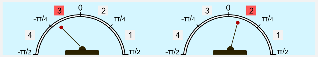
Here  , and atat is the action at time tt. The reward is updated considering the cosine of the angle , meaning larger the angle lower the reward. The reward is 0.0 when the pole is horizontal and 1.0 when vertical. When the pole is completely horizontal the episode finishes. Like in the mountain car example we can use discretization to enclose the continuous state space in pre-defined bins. For example, the position is codified with an angle in the range
 ![[\frac{-\pi}{2}, \frac{\pi}{2}]](http://www.freesandal.org/wp-content/ql-cache/quicklatex.com-9774586f3753f3cf9ff0dc4a325ab8c8_l3.png "Rendered by QuickLaTeX.com") and it can be discretized in 4 bins. When the pole has an angle of
and it can be discretized in 4 bins. When the pole has an angle of  it is in the third bin, when it has an angle of
  it is in the second bin, etc.
I wrote a special module called inverted_pendulum.py containing the classInvertedPendulum. Like in the mountain car module there are the methods reset(), step(), and render() which allow starting the episode, moving the pole and saving a gif. The animation is produced using Matplotlib and can be imagined as a camera centred on the cartpole main joint which moves in accordance with it. To create a new environment it is necessary to create a new instance of the InvertedPendulum object, defining the main parameters (masses, pole length and time step).
from inverted_pendulum import InvertedPendulum

# Defining a new environment with pre-defined parameters
my_pole = InvertedPendulum(pole_mass=2.0,
                           cart_mass=8.0,
                           pole_lenght=0.5,
                           delta_t=0.1)
We can test the performance of an agent which follows a random policy. The code is calledrandom_agent_inverted_pendulum.py and is available on the repository. Using a random strategy on the pole balancing environment leads to unsatisfactory performances. The best I got running the script multiple times is a very short episode of 1.5 seconds.
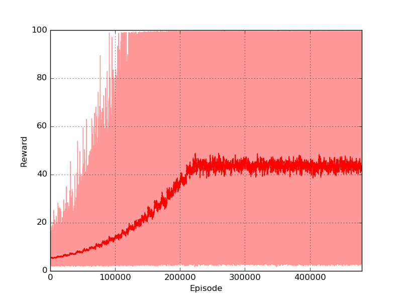
The optimal policy consists in compensating the angle and speed variations keeping the pole as much vertical as possible. Like for the mountain car I will deal with this problem using discretization. Both velocity and angle are discretized in bins of equal size and the resulting arrays are used as indices of a square policy matrix. As algorithm I will use first-visit Monte Carlo for control, which has been introduced in the second post of the series. I trained the policy for 5×1055×105 episodes (gamma=0.999, tot_bins=12). In order to encourage exploration I used an ϵϵ-greedy strategy with ϵ linearly decayed from 0.99 to 0.1. Each episode was 100 steps long (10 seconds). The maximum reward that can be obtained is 100 (the pole is kept perfectly vertical for all the steps). The reward plot shows that the algorithm could rapidly find good solutions, reaching an average score of 45.
The final policy has a very good performance and with a favourable starting position can easily manage to keep the pole in balance for the whole episode (10 seconds).
The complete code is called montecarlo_control_inverted_pendulum.py and is included in theGithub repository of the project. Feel free to change the parameters and check if they have an impact on the learning. Moreover you should test other algorithms on the pole balancing problem and verify which one gets the best performance.
啃啃學術論文︰
Non-Linear Swing-Up and Stabilizing Controlof an Inverted Pendulum System

K K 他人程式︰
Todd Sifleet
inverted pendulum
This is a video of a simulation I made with python and matplotlib. It is the standard Inverted Pendulum control problem, I implemented an LQR Controller in python-control for stabilization. To bring the pendulum from the down position to upright, I used an energy based controller. Source Code
翻翻
Library conventions
The python-control library uses a set of standard conventions for the way that different types of standard information used by the library.
LTI system representation
Linear time invariant (LTI) systems are represented in python-control in state space, transfer function, or frequency response data (FRD) form. Most functions in the toolbox will operate on any of these data types and functions for converting between between compatible types is provided.
State space systems
The StateSpace class is used to represent state-space realizations of linear time-invariant (LTI) systems:

where u is the input, y is the output, and x is the state.
To create a state space system, use the StateSpace constructor:
sys = StateSpace(A, B, C, D)
State space systems can be manipulated using standard arithmetic operations as well as thefeedback(), parallel(), and series() function. A full list of functions can be found in Function reference.
找找資料︰
control.lqr
control.lqr(A, B, Q, R[, N])- Linear quadratic regulator design
The lqr() function computes the optimal state feedback controller that minimizes the quadratic cost

The function can be called with either 3, 4, or 5 arguments:
lqr(sys, Q, R)lqr(sys, Q, R, N)lqr(A, B, Q, R)lqr(A, B, Q, R, N)
where sys is an LTI object, and A, B, Q, R, and N are 2d arrays or matrices of appropriate dimension.
Parameters: A, B: 2-d array :
Dynamics and input matrices
sys: LTI (StateSpace or TransferFunction) :
Linear I/O system
Q, R: 2-d array :
State and input weight matrices
N: 2-d array, optional :
Cross weight matrix
Returns: K: 2-d array :
State feedback gains
S: 2-d array :
Solution to Riccati equation
E: 1-d array :
Eigenvalues of the closed loop system
固能知其梗概也!
實不如按部就班讀本書好?
Feedback Systems by Karl J. Åström and Richard M. Murray
This page contains information about version 2.11b of Feedback Systems by Karl J. Åström and Richard M. Murray. Version 2.11b contains corrections to the first printing through 28 Sep 2012. This revision contains corrections to the third printing of the book.
Note: This version of the book uses a different set of fonts from the original printed book and so some pages numbers may be slightly different. Any errata reported below correspond to the location of the equivalent correction in the original printed version.
Additional info and links:
- Revision date: 28 September 2012
- Complete book – this a PDF of the entire book, as a single PDF file (408 pages, 8 MB).
- Individual chapters: P, 1, 2, 3, 4, 5, 6, 7, 8, 9, 10, 11, 12, B
- Hyperlink version – this is a PDF of the entire book, with hypertext links on references for equations, figures, citations, etc.
- iPad optimized version iPad optimized version – see the e-book page for information on how to use this file.
The electronic edition of Feedback Systems is provided with the permission of the publisher, Princeton University Press. This manuscript is for personal use only and may not be reproduced, in whole or in part, without written consent from the publisher.