


 』的一般?!已經完全不像他的『白馬非馬論』了。
洛基的賭注 Loki’s Wager
洛基乃北歐神話中以『詐騙』著名之神。傳說他曾與矮人打賭卻輸了。當矮人們依約來『提頭』時,洛基說︰『沒問題』,但是必須依照『約定』,只能取走『他的頭』,而不能動著『他的脖子』。於是彼此開始『爭論』該如何的『切割』:有哪些部分雙方同意『是頭』;又有哪些部分認同『是脖子』。只是脖子的『結束點』和頭之『開始點』究竟『是哪裡』,互相一直無法『取得共識』。於是洛基終於保住著了他的頭。
─── 《THUE 之改寫系統《二》》
考慮一個『動力系統』,將其『所受力』區分成  與
與  有道理嗎?但思自然中並非任意力都是『可控制』的 ── 比方說『重力』── !
那麼有人想要設計 □ ○ 『 控制系統』,將此系統從 □ 『初始態 』 ,變遷至意欲之 ○ 『終止態』,這人是想鎔鑄『動力』與『控制』於一爐耶??此事還請自讀文本,自觀這個思維方法所由也!!
Background
This section is intended to give some insights into the mathematical background that is the basis of PyTrajectory.
Trajectory planning with BVP’s
The task in the field of trajectory planning PyTrajectory is intended to perform, is the transition of a control system between desired states. A possible way to solve such a problem is to treat it as a two-point boundary value problem with free parameters. This approach is based on the work of K. Graichen and M. Zeitz (e.g. see [Graichen05]) and was picked up by O. Schnabel ([Schnabel13]) in the project thesis from which PyTrajectory emerged. An impressive application of this method is the swingup of the triple pendulum, see [TU-Wien-video] and [Glueck13].
Collocation Method
Given a system of autonomous differential equations
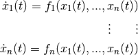
with ![t \in [a, b]](https://pytrajectory.readthedocs.io/en/master/_images/math/7ee1e80a90cec6b0dea8088399ebb8442e81fc28.png) and Dirichlet boundary conditions
and Dirichlet boundary conditions

the collocation method to solve the problem basically works as follows.
We choose ![[a, b]](https://pytrajectory.readthedocs.io/en/master/_images/math/1d2d3c2141e9f7387a2d26b1ea40c2aabd96f3ac.png) where
where 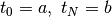 and search for functions
 ![S_i:[a,b] \rightarrow \mathbb{R}](https://pytrajectory.readthedocs.io/en/master/_images/math/9cf43e534d51d3477a6567b4cd77eee244f39c2c.png) which for all
which for all  satisfy the following conditions:
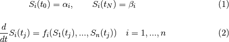
Through these demands the exact solution of the differential equation system will be approximated. The demands on the boundary values  can be sure already by suitable construction of the candidate functions. This results in the following system of equations.
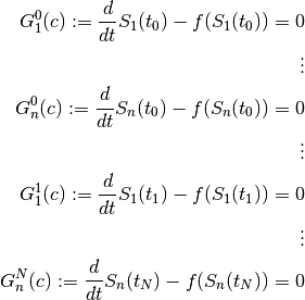
Solving the boundary value problem is thus reduced to the finding of a zero point of  , where
  is the vector of all independent parameters that result from the candidate functions.
Candidate Functions
PyTrajectory uses cubic spline functions as candidates for the approximation of the solution. Splines are piecewise polynomials with a global differentiability. The connection points  between the polynomial sections are equidistantly and are referred to as nodes.
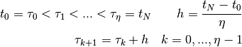
The  polynomial sections can be created as follows.
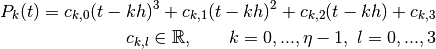
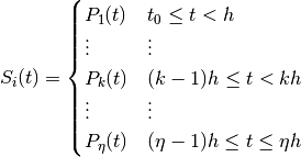
Then, each spline function is defined by
The spline functions should be twice continuously differentiable in the nodes  . Therefore, three smoothness conditions can be set up in all
 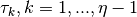 .
.
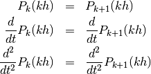
In the later equation system these demands result in the block diagonal part of the matrix. Furthermore, conditions can be set up at the edges arising from the boundary conditions of the differential equation system.

The degree  of the boundary conditions depends on the structure of the differential equation system. With these conditions and those above one obtains the following equation system (
 ).
).
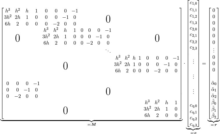
The matrix  of dimension
 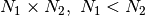 , where
  and
and  , can be decomposed into two subsystems
 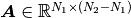 and
and  . The vectors
  and
and belong to the two matrices with the respective coefficients of
  .
.
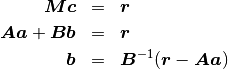
With this allocation, the system of equations can be solved for and the parameters in remain as the free parameters of the spline function.
如是也可利於自己『論理決則』乎!☆
Autonomous system (mathematics)
In mathematics, an autonomous system or autonomous differential equation is a system of ordinary differential equations which does not explicitly depend on the independent variable. When the variable is time, they are also called time-invariant systems.
Many laws in physics, where the independent variable is usually assumed to be time, are expressed as autonomous systems because it is assumed the laws of nature which hold now are identical to those for any point in the past or future.
Autonomous systems are closely related to dynamical systems. Any autonomous system can be transformed into a dynamical system[citation needed] and, using very weak assumptions[citation needed], a dynamical system can be transformed into an autonomous system[citation needed].
Definition
An autonomous system is a system of ordinary differential equations of the form

- where x takes values in n-dimensional Euclidean space and t is usually time.
It is distinguished from systems of differential equations of the form

- in which the law governing the rate of motion of a particle depends not only on the particle’s location, but also on time; such systems are not autonomous.
Properties
Let  be a unique solution of the initial value problem for an autonomous system
 .
.
Then  solves
 .
.
Indeed, denoting  we have
  and
and  , thus
 .
.
For the initial condition, the verification is trivial,
 .
.
……
邊值問題
在微分方程式中,邊值問題是一個微分方程式和一組稱之為邊界條件的約束條件。邊值問題的解通常是符合約束條件的微分方程式的解。
物理學中經常遇到邊值問題,例如波動方程式等。許多重要的邊值問題屬於Sturm-Liouville問題。這類問題的分析會和微分算子的本徵函數有關。
在實際應用中,邊值問題應當是適定的(即:存在解,解唯一且解會隨著初始值連續的變化)。許多偏微分方程式領域的理論提出是為要證明科學及工程應用的許多邊值問題都是適定問題。
最早研究的邊值問題是狄利克雷問題,是要找出調和函數,也就是拉普拉斯方程式的解,後來是用狄利克雷原理找到相關的解。
說明
邊值問題類似初值問題,邊值問題的條件是在區域的邊界上,而初值問題的條件都是在獨立變數及其導數在某一特定值時的數值(一般是定義域的下限,所以稱為初值問題)。
例如獨立變數是時間,定義域為[0,1],邊值問題的條件會是  在
在  及
及  時的數值,而初值問題的條件會是 時的 及
  之值。
之值。
若鐵棒的一端為絕對零度,另一端溫度為水的凝固點,要找到鐵棒溫度隨位置的變化即為一個邊值問題。
若問題和時間和空間都有關,邊界條件需為某一個特定點下所有時間對應的值,以及某一個特定時間時所有位置對應的值。
以下是一個邊值問題的例子

- 要求解滿足以下邊界條件的函數


- 若沒有邊界條件,以上微分方程式的通解是

- 根據邊界條件
 ,可得
,可得 
- 可以得到
 的結論。根據邊界條件
  ,可得
,可得 
- 因此
 。因此可以找到滿足上述邊界條件的唯一解,即為
-
邊值問題的種類

根據條件的形式,邊值條件分以下三類[1]:
- 第一類邊值條件:也稱為狄利克雷邊界條件,直接描述物理系統邊界上的物理量,例如振動的弦兩端與平衡位置的距離;
- 第二類邊值條件:也稱為諾伊曼邊界條件,描述物理系統邊界上物理量垂直邊界的導數的情況,例如導熱細杆端點的熱流;
- 第三類邊值條件:物理系統邊界上物理量與垂直邊界導數的線性組合,例如,細杆端點的自由冷卻,溫度、熱流均不確定,但是二者的關係確定,即可列出二者線性組合而成的邊值條件。
邊值條件也可以根據邊值問題對應的微分算子來分類:若是使用橢圓算子,則問題為橢圓邊值問題;使用雙曲線算子,則問題為雙曲線邊值問題。依微分算子還可以將問題再細分為線性及非線性等。
其餘,祇待有興趣者細究精研自能創生哩◎
Swing up of a 3-bar pendulum
Now we consider a cart with 3 pendulums attached to it.
To get a callable function for the vector field of this dynamical system we need to set up and solve its motion equations for the accelaration.
Therefore, the function n_bar_pendulum generates the mass matrix  and right hand site
  of the motion equations
  for a general
  -bar pendulum, which we use for the case
  .
.
The formulas this function uses are taken from the project report ‘Simulation of the inverted pendulum’ written by C. Wachinger, M. Pock and P. Rentrop at the Mathematics Departement, Technical University Munich in December 2004.
※ 註


……

