STEM 隨筆︰古典力學︰運動學【五‧二‧ I 】

2018-04-25 懸鉤子

公元前三八四年亞里斯多德出生於色雷斯的斯塔基拉，他是哲學家柏拉圖的學生與亞歷山大大帝的老師。他一生著作豐富，囊括了物理學、形上學、詩歌、戲劇、音樂、生物學、動物學、邏輯學、政治、政府、以及倫理學，乃西方哲學的奠基者之一。亞里斯多德的物理學思想深刻的重塑了中世紀的學術思想，其影響力之大延伸到了文藝復興時期，終被伽利略所改寫，後為牛頓物理學所取代。

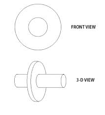
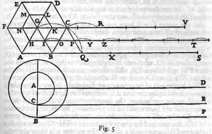
傳聞亞里斯多德著作了一本『 Mechanica or Mechanical Problems; Greek: Μηχανικά 』之力學書，這個『亞里斯多德之輪』的悖論就是出自這本書。滾動一個圓狀物，用它在平面上運動的『軌跡』就可以測量『圓周長』，這本是平凡無奇。但是左圖的動畫卻顯示，大小二圓顯然走了一樣的『距離』，難道它們的『圓周長』一樣的嗎？由歐基里德的幾何學可以知道圓周長等於『 π ‧ 直徑』，這到底是怎麼回事呢？很清楚 $\overline{AD} = \overline{BE} = \overline{CF}$ ，難道不是這樣的嗎？一六三二年伽利略用義大利文撰寫了一部天文學著作，英文譯作『關於托勒密和哥白尼兩大世界體系的對話』。在『第一天』的對話裡，他談到了『亞里斯多德之輪』︰

SALV. Otherwise what? Now since we have arrived at paradoxes let us see if we cannot prove that within a finite extent it is possible to discover an infinite number of vacua. At the same time we shall at least reach a solution of the most remarkable of all that list of problems which Aristotle himself calls wonderful; I refer to his Questions in Mechanics. This solution may be no less clear and conclusive than that which be himself gives and quite different also from that so cleverly expounded by the most learned Monsignor di Guevara.*

First it is necessary to consider a proposition, not treated by others, but upon which depends the solution of the problem and from which, if I mistake not, we shall derive other new and remarkable facts. For the sake of clearness let us draw an accurate figure. ……

……

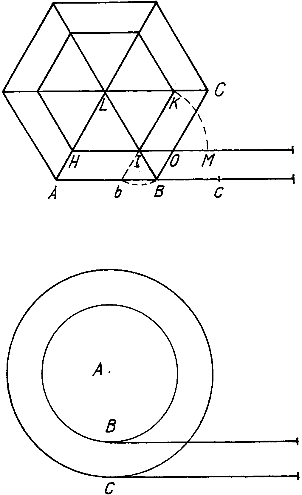
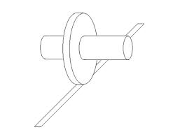
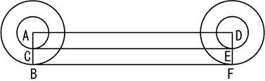
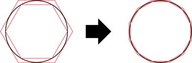
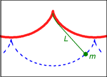
因此伽利略用『可分割』之『有限多邊形』來研究『無窮多邊』的『圓』，並說這個『有限』到『無窮』的『跳躍』是『一步到位』之『不可說』之超越。他觀察以第一圖『大』多邊形為主的每『定』點之『軌跡』，與第二圖『小』多邊形為主的各『定』點之『現象』來作比較。事實上是『大小』兩多邊形的運動軌跡不同，而且不同時間的速度也不相同。其實與平面之『接觸點』輪轉而變化，這個『想像』的『固定點』就是亞里斯多德之輪的『誤謬』來源。如果從現今的物理學來講只有『圓心』之軌跡才走『那一條』畫出的軌跡︰

如今這個『大圓』上之圓周的某個『定點』，畫出的『軌跡』稱之為『擺線』cycloid。為什麼要叫作『擺線』的呢？也許是德國的數學家 Christiaan Huygens 所發現這樣作的『鐘擺』之『準確性』和『振幅』無關，或許可以作為一種精準的時鐘？然而事實又何止是如此的呢？有人研究地球上『A、B』兩點之間運動的『最短時間』曲線；以及有人發現一條叫作 Tautochrone curve 的『同時曲線』── 各物不管原先『起始』在哪個位置，它所『到達』的時刻卻都是相同的 ── 顯示這一切或許不得不與『之』有關的吧！！

─── 《亞里斯多德之輪！！》

『輪子』之發明古早矣。從亞里斯多德到伽利略久遠也！那時『滾動現象』的物理解釋，方露曙光乎？

即使至今說明，尚覺概念沈重呦！？

Rolling

Rolling is a type of motion that combines rotation (commonly, of an axially symmetric object) and translation of that object with respect to a surface (either one or the other moves), such that, if ideal conditions exist, the two are in contact with each other without sliding.

Rolling where there is no sliding is referred to as pure rolling. By definition, there is no sliding when the instantaneous velocity of the rolling object in all the points in which it contacts the surface is the same as that of the surface; in particular, for a reference plane in which the rolling surface is at rest, the instantaneous velocity of the point of contact of the rolling object is zero.

In practice, due to small deformations near the contact area, some sliding and energy dissipation occurs. Nevertheless, the resulting rolling resistance is much lower than sliding friction, and thus, rolling objects, typically require much less energy to be moved than sliding ones. As a result, such objects will more easily move, if they experience a force with a component along the surface, for instance gravity on a tilted surface, wind, pushing, pulling, or torque from an engine. Unlike most axially symmetrical objects, the rolling motion of a cone is such that while rolling on a flat surface, its center of gravity performs a circular motion, rather than linear motion. Rolling objects are not necessarily axially-symmetrical. Two well known non-axially-symmetrical rollers are the Reuleaux triangle and the Meissner bodies. The oloid and the sphericon are members of a special family of developable rollers thatdevelop their entire surface when rolling down a flat plane. Objects with corners, such as dice, roll by successive rotations about the edge or corner which is in contact with the surface.

The animation illustrates rolling motion of a wheel as a superposition of two motions: translation with respect to the surface, and rotation around its own axis.

Applications

Most land vehicles use wheels and therefore rolling for displacement. Slip should be kept to a minimum (approximating pure rolling), otherwise loss of control and an accident may result. This may happen when the road is covered in snow, sand, or oil, when taking a turn at high speed or attempting to brake or accelerate suddenly.

One of the most practical applications of rolling objects is the use of rolling-element bearings, such as ball bearings, in rotating devices. Made of metal, the rolling elements are usually encased between two rings that can rotate independently of each other. In most mechanisms, the inner ring is attached to a stationary shaft (or axle). Thus, while the inner ring is stationary, the outer ring is free to move with very little friction. This is the basis for which almost all motors (such as those found in ceiling fans, cars, drills, etc.) rely on to operate. The amount of friction on the mechanism’s parts depends on the quality of the ball bearings and how much lubrication is in the mechanism.

Rolling objects are also frequently used as tools for transportation. One of the most basic ways is by placing a (usually flat) object on a series of lined-up rollers, or wheels. The object on the wheels can be moved along them in a straight line, as long as the wheels are continuously replaced in the front (see history of bearings). This method of primitive transportation is efficient when no other machinery is available. Today, the most practical application of objects on wheels are cars, trains, and other human transportation vehicles.

Physics of simple rolling

The velocities of the points of a rolling object are equal to those of rotation around the point of contact.

The simplest case of rolling is that of an axially symmetrical object rolling without slip along a flat surface with its axis parallel to the surface (or equivalently: perpendicular to the surface normal).

The trajectory of any point is a trochoid; in particular, the trajectory of any point in the object axis is a line, while the trajectory of any point in the object rim is a cycloid.

The velocity of any point in the rolling object is given by $\displaystyle \mathbf {v} ={\boldsymbol {\omega }}\times \mathbf {r}$ , where $\displaystyle \mathbf {r}$ is the displacement between the particle and the rolling object’s contact point (or line) with the surface, and $\displaystyle {\boldsymbol {\omega }}$ is the angular velocity vector. Thus, despite that rolling is different from rotation around a fixed axis, the instantaneous velocity of all particles of the rolling object is the same as if it was rotating around an axis that passes through the point of contact with the same angular velocity.

Any point in the rolling object farther from the axis than the point of contact will temporarily move opposite to the direction of the overall motion when it is below the level of the rolling surface (for example, any point in the part of the flange of a train wheel that is below the rail).

Energy

Since kinetic energy is entirely a function of an object mass and velocity, the above result may be used with the parallel axis theorem to obtain the kinetic energy associated with simple rolling

$\displaystyle K_{\text{rolling}}=K_{\text{translation}}+K_{\text{rotation}}$

Forces and acceleration

Differentiating the relation between linear and angular velocity, $\displaystyle v_{\text{c.o.m.}}=r\omega$ , with respect to time gives a formula relating linear and angular acceleration $\displaystyle a=r\alpha$ . Applying Newton’s second law:

$\displaystyle a={\frac {F_{\text{net}}}{m}}=r\alpha ={\frac {r\tau }{I}}.$

It follows that to accelerate the object, both a net force and a torque are required. When external force with no torque acts on the rolling object‐surface system, there will be a tangential force at the point of contact between the surface and rolling object that provides the required torque as long as the motion is pure rolling; this force is usually static friction, for example, between the road and a wheel or between a bowling lane and a bowling ball. When static friction isn’t enough, the friction becomes dynamic friction and slipping happens. The tangential force is opposite in direction to the external force, and therefore partially cancels it. The resulting net force and acceleration are:

$\displaystyle F_{\text{net}}={\frac {F_{\text{external}}}{1+{\frac {I}{mr^{2}}}}}={\frac {F_{\text{external}}}{1+\left({\frac {r_{\text{gyr.}}}{r}}\right)^{2}}}$

$\displaystyle a={\frac {F_{\text{external}}}{m+{\frac {I}{r^{2}}}}}$

\displaystyle {\tfrac {I}{r^{2}}}

has dimension of mass, and it is the mass that would have a rotational inertia $\displaystyle I$ at distance $\displaystyle r$ from an axis of rotation. Therefore, the term $\displaystyle {\tfrac {I}{r^{2}}}$ may be thought of as the mass with linear inertia equivalent to the rolling object rotational inertia (around its center of mass). The action of the external force upon an object in simple rotation may be conceptualized as accelerating the sum of the real mass and the virtual mass that represents the rotational inertia, which is $\displaystyle m+{\tfrac {I}{r^{2}}}$ . Since the work done by the external force is split between overcoming the translational and rotational inertia, the external force results in a smaller net force by the dimensionless multiplicative factor $\displaystyle 1/\left(1+{\tfrac {I}{mr^{2}}}\right)$ where $\displaystyle {\tfrac {I}{mr^{2}}}$ represents the ratio of the aforesaid virtual mass to the object actual mass and it is equal to $\displaystyle \left({\tfrac {r_{\text{gyr.}}}{r}}\right)^{2}$ where $\displaystyle r_{\text{gyr.}}$ is the radius of gyration corresponding to the object rotational inertia in pure rotation (not the rotational inertia in pure rolling). The square power is due to the fact that the rotational inertia of a point mass varies proportionally to the square of its distance to the axis.

Four objects in pure rolling racing down a plane with no air drag. From back to front: spherical shell (red), solid sphere (orange), cylindrical ring (green) and solid cylinder (blue). The time to reach the finishing line is entirely a function of the object mass distribution, slope and gravitational acceleration. See details, animated GIF version.

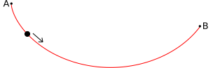
In the specific case of an object rolling in an inclined plane which experiences only static friction, normal force and its own weight, (air drag is absent) the acceleration in the direction of rolling down the slope is:

$\displaystyle a={\frac {g\sin \left(\theta \right)}{1+\left({\tfrac {r_{\text{gyr.}}}{r}}\right)^{2}}}$

$\displaystyle {\tfrac {r_{\text{gyr.}}}{r}}$ is specific to the object shape and mass distribution, it does not depends on scale or density. However, it will vary if the object is made to roll with different radiuses; for instance, it varies between a train wheel set rolling normally (by its tire), and by its axle. It follows that given a reference rolling object, another object bigger or with different density will roll with the same acceleration. This behavior is the same as that of an object in free fall or an object sliding without friction (instead of rolling) down an inclined plane.

欲假 SymPy mechanics 的

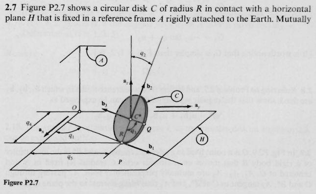
A rolling disc

The disc is assumed to be infinitely thin, in contact with the ground at only 1 point, and it is rolling without slip on the ground. See the image below.

We model the rolling disc in three different ways, to show more of the functionality of this module.

範例說說 □ ○ 方法之事，偏偏圖示過簡的呀？！

不得已借道

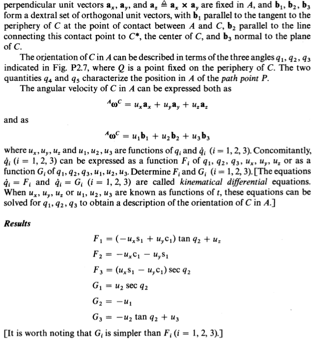
“””Exercise 2.7 from Kane 1985″””

，先有個確切描述吧！！

樹莓派、樹莓派之學習、樹莓派之教育

STEM 隨筆︰古典力學︰運動學【五‧一】

2018-04-24 懸鉤子

或許當文章順暢說明簡單，人的思維容易被牽著鼻子走乎？

故耳有時須跳脫其境旁敲側擊也，如是方可直抵關鍵處呦！

Kinematic chain

In mechanical engineering, a kinematic chain is an assembly of rigid bodies connected by joints to provide constrained (or desired) motion that is the mathematical model for a mechanical system.^[1] As in the familiar use of the word chain, the rigid bodies, or links, are constrained by their connections to other links. An example is the simple open chain formed by links connected in series, like the usual chain, which is thekinematic model for a typical robot manipulator.^[2]

Mathematical models of the connections, or joints, between two links are termed kinematic pairs. Kinematic pairs model the hinged and sliding joints fundamental to robotics, often called lower pairs and the surface contact joints critical to cams and gearing, called higher pairs. These joints are generally modeled as holonomic constraints. A kinematic diagram is a schematic of the mechanical system that shows the kinematic chain.

The modern use of kinematic chains includes compliance that arises from flexure joints in precision mechanisms, link compliance in compliant mechanisms and micro-electro-mechanical systems, and cable compliance in cable robotic and tensegrity systems.^[3] ^[4]

Mobility formula

The degrees of freedom, or mobility, of a kinematic chain is the number of parameters that define the configuration of the chain.^[2]^[5] A system of n rigid bodies moving in space has 6n degrees of freedom measured relative to a fixed frame. This frame is included in the count of bodies, so that mobility does not depend on link that forms the fixed frame. This means the degree-of-freedom of this system is M = 6(N − 1), whereN = n + 1 is the number of moving bodies plus the fixed body.

Joints that connect bodies impose constraints. Specifically, hinges and sliders each impose five constraints and therefore remove five degrees of freedom. It is convenient to define the number of constraints c that a joint imposes in terms of the joint’s freedom f, where c = 6 − f. In the case of a hinge or slider, which are one degree of freedom joints, have f = 1 and therefore c = 6 − 1 = 5.

The result is that the mobility of a kinematic chain formed from n moving links and j joints each with freedom f_i, i = 1, …, j, is given by

$\displaystyle M=6n-\sum _{i=1}^{j}(6-f_{i})=6(N-1-j)+\sum _{i=1}^{j}f_{i}$

Recall that N includes the fixed link.

Analysis of kinematic chains

The constraint equations of a kinematic chain couple the range of movement allowed at each joint to the dimensions of the links in the chain, and form algebraic equations that are solved to determine the configuration of the chain associated with specific values of input parameters, called degrees of freedom.

The constraint equations for a kinematic chain are obtained using rigid transformations [Z] to characterize the relative movement allowed at each joint and separate rigid transformations [X] to define the dimensions of each link. In the case of a serial open chain, the result is a sequence of rigid transformations alternating joint and link transformations from the base of the chain to its end link, which is equated to the specified position for the end link. A chain of n links connected in series has the kinematic equations,

$\displaystyle [T]=[Z_{1}][X_{1}][Z_{2}][X_{2}]\cdots [X_{n-1}][Z_{n}],\!$

where [T] is the transformation locating the end-link—notice that the chain includes a “zeroth” link consisting of the ground frame to which it is attached. These equations are called the forward kinematics equations of the serial chain.^[6]

Kinematic chains of a wide range of complexity are analyzed by equating the kinematics equations of serial chains that form loops within the kinematic chain. These equations are often called loop equations.

The complexity (in terms of calculating the forward and inverse kinematics) of the chain is determined by the following factors:

Its topology: a serial chain, a parallel manipulator, a tree structure, or a graph.
Its geometrical form: how are neighbouring joints spatially connected to each other?

Explanation

Two or more rigid bodies in space are collectively called a rigid body system. We can hinder the motion of these independent rigid bodies with kinematic constraints. Kinematic constraints are constraints between rigid bodies that result in the decrease of the degrees of freedom of rigid body system.^[5]

The movement of the Boulton & Watt steam engineis studied as a system of rigid bodies connected by joints forming a kinematic chain.

Synthesis of kinematic chains

The constraint equations of a kinematic chain can be used in reverse to determine the dimensions of the links from a specification of the desired movement of the system. This is termed kinematic synthesis.^[7]

Perhaps the most developed formulation of kinematic synthesis is for four-bar linkages, which is known as Burmester theory.^[8]^[9]^[10]

Ferdinand Freudenstein is often called the father of modern kinematics for his contributions to the kinematic synthesis of linkages beginning in the 1950s. His use of the newly developed computer to solve Freudenstein’s equation became the prototype of computer-aided design systems.^[7]

This work has been generalized to the synthesis of spherical and spatial mechanisms.^[2]

A model of the human skeleton as a kinematic chain allows positioning using forward and inverse kinematics.

無論想象力可否聞一知十耶？？

Four-bar linkage

From Wikipedia, the free encyclopedia

A four-bar linkage, also called a four-bar, is the simplest movable closed chain linkage. It consists of four bodies, called bars or links, connected in a loop by four joints. Generally, the joints are configured so the links move in parallel planes, and the assembly is called a planar four-bar linkage. Spherical and spatial four-bar linkages also exist and they are used in practice. ^[1]

Pumpjacks’ main mechanism is a four-bar linkage

Planar four-bar linkage

Planar four-bar linkages are constructed from four links connected in a loop by four one-degree-of-freedom joints. A joint may be either a revolute, that is a hinged joint, denoted by R, or a prismatic, as sliding joint, denoted by P.

A link connected to ground by a hinged joint is usually called a crank. A link connected to ground by a prismatic joint is called a slider. Sliders are sometimes considered to be cranks that have a hinged pivot at an extremely long distance away perpendicular to the travel of the slider.

The link that connects two cranks is called a floating link or coupler. A coupler that connects a crank and a slider, it is often called a connecting rod.

There are three basic types of planar four-bar linkage depending on the use of revolute or prismatic joints:

Four revolute joints: The planar quadrilateral linkage is formed by four links and four revolute joints, denoted RRRR. It consists of two cranks connected by a coupler.
Three revolute joints and a prismatic joint: The slider-crank linkage is constructed from four links connected by three revolute and one prismatic joint, or RRRP. It can be constructed with crank and a slider connected by the connecting rod. Or it can be constructed as a two cranks with the slider acting as the coupler, known as an inverted slider-crank.
Two revolute joints and two prismatic joints: The double slider is a PRRP linkage.^[2] This linkage is constructed by connecting two sliders with a coupler link. If the directions of movement of the two sliders are perpendicular then the trajectories of the points in the coupler are ellipses and the linkage is known as an elliptical trammel, or the Trammel of Archimedes.

Planar four-bar linkages are important mechanisms found in machines. The kinematics and dynamics of planar four-bar linkages are important topics in mechanical engineering.

Planar four-bar linkages can be designed to guide a wide variety of movements.

Coupler curves of a crank-rocker four-bar linkage. Simulation done with MeKin2D.

且求自能問又自能答矣！！

樹莓派、樹莓派之學習、樹莓派之教育

STEM 隨筆︰古典力學︰運動學【五】

2018-04-23 懸鉤子

因為牛頓力學之運動方程『形式』假設了『慣性觀察者』。即使無視『接近光速』的『特殊相對論』，所謂『三體問題』

Three-body problem

In physics and classical mechanics, the three-body problem is the problem of taking an initial set of data that specifies the positions, masses, and velocities of three bodies for some particular point in time and then determining the motions of the three bodies, in accordance with Newton’s laws of motion and of universal gravitation which are the laws of classical mechanics. The three-body problem is a special case of the $n$ -body problem. Unlike two-body problems, there is no general closed-form solution for every condition, and numerical methods are needed to solve these problems.

Historically, the first specific three-body problem to receive extended study was the one involving the Moon, the Earth, and the Sun.^[1] In an extended modern sense, a three-body problem is a class of problems in classical or quantum mechanics that models the motion of three particles.

尚且難得『數學確解』也！如何能說 $N$ 個『質點』之問題呢？

因此大千萬象、日常物體的『運動描述』豈非無望耶？？

故而『理想假設』之興，求其近似，易於『計算推導』矣！！

剛體運動學

剛體的空間位形決定於其質心位置與其取向（最多有六個自由度）。^[4]

主條目：剛體運動學

在物理學裏，理想剛體是一種有限尺寸，可以忽略形變的固體。不論是否感受到外力，在剛體內部，點與點之間的距離都不會改變。根據相對論，這種物體不可能實際存在，但物體通常可以假定為完美剛體，前提是必須滿足運動速度超小於光速的條件。

剛體是由一群數量超多的質點組成。實際而言，不可能精確地追蹤其中每一個質點的運動。為了簡化運算，通常，整個剛體的空間位形可以簡易地以參數設定：

剛體的「位置」：挑選剛體內部一點 G 來代表整個剛體，通常會設定物體的質心或形心為這一點。從空間參考系 S 觀測，點 G 的位置就是整個剛體在空間的位置。位置可以應用向量的概念來表示：向量的起點為參考系 S 的原點，終點為點 G 。
剛體的取向：描述剛體取向的方法有好幾種，包括方向餘弦、歐拉角、四元數等等。這些方法設定一個附體參考系 B 的取向（相對於空間參考系 S ）。附體參考系是固定於剛體的參考系。相對於剛體，附體參考系的取向固定不變。由於剛體可能會呈加速度運動，所以附體參考系可能不是慣性參考系。空間參考系是某設定慣性參考系，例如，在觀測飛機的飛行運動時，附著於飛機場控制塔的參考系可以設定為空間參考系，而附著於飛機的參考系則可設定為附體參考系。

歐拉旋轉定理

歐拉旋轉定理表明，在三維空間裏，假設約束剛體內部一點固定不動，則其任意位移等價於繞著某固定軸的一個旋轉，而這固定軸必包含這固定點。換句話說，設定附體參考系 B 的原點為這固定點，則附體參考系 B 不會因為這位移而涉及任何平移運動，這位移等價於繞著某固定軸的一個旋轉。^[2]

沙勒定理

剛體平移運動示意圖。

當剛體移動時，它的位置與取向都可能會隨著時間演進而改變。沙勒定理是歐拉旋轉定理的一個推論。根據沙勒定理，剛體的最廣義位移等價於一個平移加上一個旋轉。^[2]因此，剛體運動可分為平移運動與旋轉運動。剛體的現在位置與現在取向可以視為是從某個初始位置與初始取向經過平移與旋轉而成。

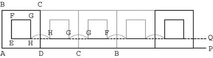
如右圖所示，從時間 $\displaystyle t_{1}$ 到時間 $\displaystyle t_{2}$ ，當剛體在做平移運動時，任意內部兩點，點 P 與點 Q 的軌跡（以黑色實線表示）相互平行，線段 $\displaystyle {\overline {PQ}}$ （以黑色虛線表示）的方向保持恆定。

挑選剛體內部一點 G 來代表整個剛體，設定附體參考系 B 的原點於點 G （稱為「基點」），則從空間參考系 S 觀測，在剛體內部任意一點 P 的位置 $\displaystyle \mathbf {r} _{P}$ 為

$\displaystyle \mathbf {r} _{P}=\mathbf {r} _{G}+\mathbf {r} _{P/G}$ ；

其中， $\displaystyle \mathbf {r} _{G}$ 分別是基點 G 的位置、點 P 對於基點 G 的相對位置。

從附體參考系 B 觀測，剛體內部每一點的位置都固定不變，但從空間參考系 S 觀測，剛體從時間 $\displaystyle t_{1}$ 到時間 $\displaystyle t_{2}$ 的運動，可以分為基點 G 從 $\displaystyle \mathbf {r} _{G}(t_{1})$ 到 $\displaystyle \mathbf {r} _{G}(t_{2})$ 的平移運動，與位移 $\displaystyle \mathbf {r} _{P/G}$ 從時間 $\displaystyle t_{1}$ 到時間 $\displaystyle t_{2}$ 的旋轉運動。

平移速度與角速度

從不同的參考系觀測剛體運動，可能會獲得不同的平移速度和不同的角速度。為了確保測量結果具有實際物理意義，必需先給定參考系。

剛體的平移速度是向量，是其位置向量的時間變化率，是附著於剛體的基點 G 的速度。對於純平移運動（沒有任何旋轉運動），剛體內部所有點的移動速度相同。假設涉及旋轉運動，則通常剛體內部任意兩點的瞬時速度不相等；只有當它們恰巧處於同一直軸，而這直軸平行於轉動瞬軸，則它們的瞬時速度相等。

角速度也是向量，描述剛體取向改變的角速率，和剛體旋轉時的瞬時轉軸的方向（歐拉旋轉定理保證瞬時轉軸的存在）。在任意時間，剛體內部每一個質點的角速度相同。

向量的時間變化率

假設一剛體呈純旋轉運動，旋轉的角速度為 $\displaystyle {\boldsymbol {\omega }}$ ，其附體參考系 B 也會跟著旋轉，因此，對於任意向量 $\displaystyle \mathbf {F}$ ，從這附體參考系 B 與從空間參考系 S 觀測，會得到不同的結果。設定

$\displaystyle \left({\frac {\mathrm {d} \mathbf {F} }{\mathrm {d} t}}\right)_{\mathrm {space} }$ 、 $\displaystyle \left({\frac {\mathrm {d} \mathbf {F} }{\mathrm {d} t}}\right)_{\mathrm {body} }$ 分別為從空間參考系 S 、附體參考系 B 觀測到的向量 $\displaystyle \mathbf {F} (t)$ 對於時間的導數，則

$\displaystyle \left({\frac {\mathrm {d} \mathbf {F} }{\mathrm {d} t}}\right)_{\mathrm {space} }=\left({\frac {\mathrm {d} \mathbf {F} }{\mathrm {d} t}}\right)_{\mathrm {body} }+{\boldsymbol {\omega }}\times \mathbf {F}$ 。

項目 $\displaystyle {\boldsymbol {\omega }}\times \mathbf {F}$ 可以想像為，從空間參考系 S 觀測，剛體內部位置向量為 $\displaystyle \mathbf {F}$ 的質點，由於剛體旋轉而產生的角速度。

向量 $\displaystyle \mathbf {F} (t)$ 是任意向量，因此可以將 $\displaystyle \left({\frac {\mathrm {d} }{\mathrm {d} t}}\right)_{\mathrm {space} }$ 、 $\displaystyle \left({\frac {\mathrm {d} }{\mathrm {d} t}}\right)_{\mathrm {body} }$ 當作算符，這樣，對應的算符方程式的形式為：

$\displaystyle \left({\frac {\mathrm {d} }{\mathrm {d} t}}\right)_{\mathrm {space} }=\left({\frac {\mathrm {d} }{\mathrm {d} t}}\right)_{\mathrm {body} }+{\boldsymbol {\omega }}\times$ 。

這算符方程式可以作用於任意含時向量。

運動學方程式

根據沙勒定理，剛體的最廣義位移等價於一個平移加上一個旋轉。^[2]挑選剛體內部一點 G 來代表整個剛體，設定附體參考系 B 的原點於基點 G ，則從空間參考系 S 觀測，在剛體內部任意一點 P 的位置 $\displaystyle \mathbf {r} _{P}$ 為

$\displaystyle \mathbf {r} _{P}=\mathbf {r} _{G}+\mathbf {r} _{P/G}$ ；

其中， $\displaystyle \mathbf {r} _{G}$ 、 $\displaystyle \mathbf {r} _{P/G}$ 分別是基點 G 的位置、點 P 對於基點 G 的相對位置。

點 P 的速度 $\displaystyle \mathbf {v} _{P}=\left({\frac {\mathrm {d} \mathbf {r} _{P}}{\mathrm {d} t}}\right)_{\mathrm {space} }$ 為

$\displaystyle \mathbf {v} _{P}=\mathbf {v} _{G}+\mathbf {v} _{P/G}$ ；

其中， $\displaystyle \mathbf {v} _{G}=\left({\frac {\mathrm {d} \mathbf {r} _{G}}{\mathrm {d} t}}\right)_{\mathrm {space} }$ 、 $\displaystyle \mathbf {v} _{P/G}=\left({\frac {\mathrm {d} \mathbf {r} _{P/G}}{\mathrm {d} t}}\right)_{\mathrm {space} }$ 分別是基點 G 的速度、點 P 對於基點 G 的相對速度。

應用前段推導出的適用於任意含時向量的算符方程式，可以計算出 $\displaystyle \mathbf {v} _{P/G}$ 。由於從附體參考系 B 觀測，剛體內部每一點的位置都固定不變，項目

$\displaystyle \left({\frac {\mathrm {d} \mathbf {r} _{P/G}}{\mathrm {d} t}}\right)_{\mathrm {body} }$ 等於零：

$\displaystyle \mathbf {v} _{P/G}=\left({\frac {\mathrm {d} \mathbf {r} _{P/G}}{\mathrm {d} t}}\right)_{\mathrm {body} }+{\boldsymbol {\omega }}\times \mathbf {r} _{P/G}={\boldsymbol {\omega }}\times \mathbf {r} _{P/G}$ ;

其中， $\displaystyle {\boldsymbol {\omega }}$ 是剛體的角速度向量。

所以，點 P 的速度為

$\displaystyle \mathbf {v} _{P}=\mathbf {v} _{G}+{\boldsymbol {\omega }}\times \mathbf {r} _{P/G}$ 。

點 P 的加速度 $\displaystyle \mathbf {a} _{P}=\left({\frac {\mathrm {d} \mathbf {v} _{P}}{\mathrm {d} t}}\right)_{\mathrm {space} }$ 為

$\displaystyle \mathbf {a} _{P}=\mathbf {a} _{G}+\mathbf {a} _{P/G}$ ；

其中， $\displaystyle \mathbf {a} _{G}=\left({\frac {\mathrm {d} \mathbf {v} _{G}}{\mathrm {d} t}}\right)_{\mathrm {space} }$ 、 $\displaystyle \mathbf {a} _{P/G}=\left({\frac {\mathrm {d} \mathbf {v} _{P/G}}{\mathrm {d} t}}\right)_{\mathrm {space} }$ 分別是基點 G 的加速度、點 P 對於基點 G 的相對加速度。

再應用前段推導出的算符方程式，可以計算出

$\displaystyle \mathbf {a} _{P/G}=\left({\frac {\mathrm {d} {\boldsymbol {\omega }}}{\mathrm {d} t}}\right)_{\mathrm {space} }\times \mathbf {r} _{P/G}+{\boldsymbol {\omega }}\times \mathbf {v} _{P/G}={\boldsymbol {\alpha }}\times \mathbf {r} _{P/G}+{\boldsymbol {\omega }}\times ({\boldsymbol {\omega }}\times \mathbf {r} _{P/G})$ ；

其中， $\displaystyle {\boldsymbol {\alpha }}=\left({\frac {\mathrm {d} {\boldsymbol {\omega }}}{\mathrm {d} t}}\right)_{\mathrm {space} }$ 是附體參考系 B 旋轉的角加速度向量。

運動約束

「運動約束」指的是一個動態系統的運動必須符合的約束條件。以下列出一些例子：

純滾動

假若，一個圓柱形物體滾動於平面上，不做任何滑動運動（物體與平面之間，沒有任何滑動摩擦），則這物體的運動稱為「純滾動」，其質心的速度 $\displaystyle \mathbf {v} _{cm}$ 必須符合約束條件：

$\displaystyle \mathbf {v} _{cm}={\boldsymbol {\omega }}\times \mathbf {r} _{cm/O}$ ；

其中， $\displaystyle {\boldsymbol {\omega }}$ 是旋轉的角速度， $\displaystyle \mathbf {r} _{cm/O}$ 是從物體與平面的接觸點到物體質心的位移向量。

對於物體在滾動時不傾斜或不轉彎的案例，這約束條件約化為

$\displaystyle v=r_{cm/O}\omega$ 。

無伸縮性繩子

簡單擺的繩子長度保持不變。

當感受到張力的作用時，「無伸縮性繩子」不會因為張力的大小而改變繩子的長度。對於涉及無伸縮性繩子的物理問題，約束條件是繩子長度保持不變^[5]。

單擺：將一根無伸縮性繩子的一端固定，另外一端繫住一個錘。這就形成了一個簡單擺。在基礎動力學裏，簡單擺問題研究錘的擺動運動跟繩子長度、錘重量之間的關係。
溜溜球：在兩片圓盤之間連結的捲軸，繫著一根無伸縮性繩子。這就是古今中外、廣為流行的溜溜球玩具。
懸鏈線：將無伸縮性繩子的兩端分別固定於兩點，由於均勻重力作用於繩子的每一部份而形成的曲線形狀稱為懸鏈線^[6]。

那麼 SymPy 裡的

RigidBody

class sympy.physics.mechanics.rigidbody.RigidBody(name, masscenter, frame, mass, inertia)

An idealized rigid body.

This is essentially a container which holds the various components which describe a rigid body: a name, mass, center of mass, reference frame, and inertia.

All of these need to be supplied on creation, but can be changed afterwards.

Attributes

name	(string) The body’s name.
masscenter	(Point) The point which represents the center of mass of the rigid body.
frame	(ReferenceFrame) The ReferenceFrame which the rigid body is fixed in.
mass	(Sympifyable) The body’s mass.
inertia	((Dyadic, Point)) The body’s inertia about a point; stored in a tuple as shown above.

『程式建制』能出其右乎！！？？

誠如

n03_kinematics.ipynb

簡介所言

單講『描述複雜』亦難矣哉？？！！

樹莓派、樹莓派之學習、樹莓派之教育

STEM 隨筆︰古典力學︰運動學【四‧E】

2018-04-22 懸鉤子

俗話說︰千里來龍，在此結穴。

且讓我們借 $A$ 參考系，用 $\theta$ 角為變數，將

Nonminimal Coordinates Pendulum

In this example we demonstrate the use of the functionality provided in mechanics for deriving the equations of motion (EOM) for a pendulum with a nonminimal set of coordinates. As the pendulum is a one degree of freedom system, it can be described using one coordinate and one speed (the pendulum angle, and the angular velocity respectively). Choosing instead to describe the system using the $x$ and $y$ coordinates of the mass results in a need for constraints. The system is shown below:

The system will be modeled using both Kane’s and Lagrange’s methods, and the resulting EOM linearized. While this is a simple problem, it should illustrate the use of the linearization methods in the presence of constraints.

文本改寫一番

如是當能品味異同也！

撞日趁興何不一鼓作氣玩轉

Pendulum on a movable support

Sketch of the situation with definition of the coordinates (click to enlarge)

Consider a pendulum of mass m and length ℓ, which is attached to a support with mass M, which can move along a line in the x-direction. Let x be the coordinate along the line of the support, and let us denote the position of the pendulum by the angle θ from the vertical. The coordinates and velocity components of the pendulum bob are

$\displaystyle {\begin{array}{rll}&x_{\mathrm {pend} }=x+\ell \sin \theta &\quad \Rightarrow \quad {\dot {x}}_{\mathrm {pend} }={\dot {x}}+\ell {\dot {\theta }}\cos \theta \\&y_{\mathrm {pend} }=-\ell \cos \theta &\quad \Rightarrow \quad {\dot {y}}_{\mathrm {pend} }=\ell {\dot {\theta }}\sin \theta \end{array}}$

The generalized coordinates can be taken to be x and θ. The kinetic energy of the system is then

$\displaystyle T={\frac {1}{2}}M{\dot {x}}^{2}+{\frac {1}{2}}m\left({\dot {x}}_{\mathrm {pend} }^{2}+{\dot {y}}_{\mathrm {pend} }^{2}\right)$

and the potential energy is

$\displaystyle V=mgy_{\mathrm {pend} }$

giving the Lagrangian

$\displaystyle {\begin{array}{rcl}L&=&T-V\\&=&{\frac {1}{2}}M{\dot {x}}^{2}+{\frac {1}{2}}m\left[\left({\dot {x}}+\ell {\dot {\theta }}\cos \theta \right)^{2}+\left(\ell {\dot {\theta }}\sin \theta \right)^{2}\right]+mg\ell \cos \theta \\&=&{\frac {1}{2}}\left(M+m\right){\dot {x}}^{2}+m{\dot {x}}\ell {\dot {\theta }}\cos \theta +{\frac {1}{2}}m\ell ^{2}{\dot {\theta }}^{2}+mg\ell \cos \theta \end{array}}$

Since x is absent from the Lagrangian, it is a cyclic coordinate. The conserved momentum is

$\displaystyle p_{x}={\frac {\partial L}{\partial {\dot {x}}}}=(M+m){\dot {x}}+m\ell {\dot {\theta }}\cos \theta \,.$

and the Lagrange equation for the support coordinate x is

$\displaystyle (M+m){\ddot {x}}+m\ell {\ddot {\theta }}\cos \theta -m\ell {\dot {\theta }}^{2}\sin \theta =0$

The Lagrange equation for the angle θ is

$\displaystyle {\frac {\mathrm {d} }{\mathrm {d} t}}\left[m({\dot {x}}\ell \cos \theta +\ell ^{2}{\dot {\theta }})\right]+m\ell ({\dot {x}}{\dot {\theta }}+g)\sin \theta =0;$

and simplifying

$\displaystyle {\ddot {\theta }}+{\frac {\ddot {x}}{\ell }}\cos \theta +{\frac {g}{\ell }}\sin \theta =0.$

These equations may look quite complicated, but finding them with Newton’s laws would have required carefully identifying all forces, which would have been much more laborious and prone to errors. By considering limit cases, the correctness of this system can be verified: For example, $\displaystyle {\ddot {x}}\to 0$ should give the equations of motion for a simple pendulum that is at rest in some inertial frame, while $\displaystyle {\ddot {\theta } \to 0$ should give the equations for a pendulum in a constantly accelerating system, etc. Furthermore, it is trivial to obtain the results numerically, given suitable starting conditions and a chosen time step, by stepping through the results iteratively.

乎？

樹莓派、樹莓派之學習、樹莓派之教育

STEM 隨筆︰古典力學︰運動學【四‧D】

2018-04-21 懸鉤子

伽利略、克卜勒與潮汐理論

紅衣主教貝拉明^[48]1615年發表聲明，稱哥白尼學說不成立，除非「有物理證據證明太陽不是圍繞地球，而是地球圍繞著太陽運行」^[49]。伽利略認為他的潮汐理論足可證明地球運動。這個理論十分重要，以至於他最開始將著作命名為《關于海洋潮汐與流動的兩大世界體系的對話》^[50]。關於潮汐的字眼最終因為宗教法庭的指令而被刪除。

伽利略認為，由於地球圍繞軸心自轉並圍繞太陽公轉，導致地球表面運動的加速減速引發海水潮汐式前後涌動。1616年，他將第一份有關潮汐的文獻整理出來，交給了紅衣主教奧斯尼^[51]^[52]。他的理論第一次涉及了海底大陸架的形狀尺度，以及潮汐的時刻等。例如，他正確地推算出亞德里亞海中途的波浪相對於到達海岸的最後一波來說可以忽略不計。但是，從潮汐形成的總體角度來看，伽利略的理論並不成立。

如果理論成立了，那麼每天只能出現一次漲潮。伽利略與他的同事們注意到該理論的不足之處，因為在威尼斯每天會漲潮兩次，時間間隔為12小時。伽利略認為這種反常現象不過是因為海洋形狀，深度及其它的問題導致的^[53]，不值得一提。對於他這種觀點是不可信賴的論斷，阿爾伯特·愛因斯坦則表示伽利略只是急於給出地球運動的物理證明，構造出了這種「引人入勝的觀點」並自己全盤接受了^[54]。伽利略否定了當時約翰內斯·克卜勒的觀點，即月球導致潮汐運動^[55]，而後者的觀點襲承了托勒密法之書中占星傳統。他也拒絕接受克卜勒關於行星沿橢圓軌道運行的觀點，認為圓形軌道才是「完美」的^[56]。

─── 摘自《伽利略·伽利萊》

閱讀

潮汐

潮汐是地球上的海洋表面受到太陽和月球的萬有引力（潮汐力）作用引起的漲落現象^[1]^[2]^[3]。潮汐的變化與地球、太陽和月球的相對位置有關，並且會與地球自轉的效應耦合和海洋的海水深度、大湖及河口^[4]。在其它引力場的時間和空間系統內也會發生類似潮汐的現象。

在淺海和港灣實際發生的海平面變化，不僅受到天文的潮汐力影響，還會受到氣象（風和氣壓）的強烈影響，例如風暴潮。潮汐造成海洋和港灣口積水深度的改變，並且形成震盪的潮汐流，因此製作沿海地區潮汐流的預測在航海上是很重要的。在漲潮時會埋在海水中，而在退潮時會裸露出來的潮間帶，是潮汐造成的重要海洋生態。

……

物理學

參見：潮汐力和潮汐理論

圖5：從北極鳥瞰的地球和月球。

潮汐物理學的歷史

牛頓在他的自然哲學的數學原理（1687）一書中以科學的研究奠定了用數學解釋潮汐發生的基礎力量^[16]^[17]。牛頓首先應用牛頓萬有引力定律計算由太陽和月球吸引造成的潮汐^[18]，並且提供了引潮力最初的理論。但是牛頓的理論和他的後繼者是採用之前拉普拉斯的均衡理論，在很大的程度上是以近似值描述潮汐即使在覆蓋整個地球的非慣性海洋中也會發生^[16]引潮力（或是相當於位能）對潮汐理論依然是有意義的，但做為一個中間的數值，而不是最終的結果；理論已經考慮地球動力學與潮汐的關係，而受到地形、地Ë球自轉和其它因素的影響^[19]。

在1740年，在巴黎的法國皇家科學院提供獎金給最佳的潮汐理論，由丹尼爾·伯努利、Antoine Cavalleri、歐拉、和柯林·馬克勞林共享這筆獎金。

馬克勞林使用牛頓的理論顯示一個覆蓋了足夠深度海洋的單一平滑球體，在潮汐力的作用下會變形成為扁長的橢球體，而長軸就指向引起變形的天體。馬克勞林也是第一個寫下地球的柯里奧利力對運動的影響。

歐拉意識到在水平方向的力（引潮力）才是驅動潮汐的力（比垂直方向的起潮力大）。

在1744年，達朗貝爾研究潮汐的大氣方程式，但沒有包括轉動的因素。

皮埃爾-西蒙·拉普拉斯以偏微分方程的形式制訂有關海洋在水平的流動和海表面高度的系統，是第一件主要的潮汐動力理論，而且拉普拉斯潮汐方程在今天仍在使用。William Thomson, 1st Baron Kelvin重寫了拉普拉斯方程中的渦度項目，使方程式可以描述與解決驅動沿岸陷落波，也就是所知的克耳文波^[20] ^[21] ^[22]。

其他人，包括克耳文與亨利·龐加萊繼續開發拉普拉斯理論，根據這些發展與E W布朗和Arthur Thomas Doodson的月球理論在1921年開發和發布^[23]，第一個現代化的引潮諧波形式：道森列出了388項潮汐頻率^[24]，其中有些方法現在仍被使用著^[25]。

力

若以月球潮汐為例，作用於每單位質量的引潮力是月球的引力場在該單位質量的位置和在地心的矢量差。此每單位質量引潮力可分解為垂直 (即徑向) 分量 $\displaystyle T_{v}$ 和水平 (即切向) 分量 $\displaystyle T_{h}$ 。簡化後，它們分別是

$\displaystyle T_{v}={\frac {GmR}{D^{3}}}(3\cos ^{2}\theta -1)$ 和 $\displaystyle T_{h}={\frac {3GmR}{2D^{3}}}\sin 2\theta$ 。

其中 $\displaystyle G$ 是萬有引力常數， $\displaystyle m$ 是月球質量， $\displaystyle R$ 是地球半徑， $\displaystyle D$ 是地心與月心的距離， $\displaystyle \theta$ 是該單位質量與地心的連線與地—月連線的夾角。

最高潮發生在正面向月球 ( $\displaystyle \theta =0^{0}$ ) 和正背向月球 ( $\displaystyle \theta =180^{0}$ ) 兩位置。在該兩處 $\displaystyle T_{v}={\frac {2GmR}{D^{3}}}$ 及 $\displaystyle T_{h}=0$ 。最低潮則發生在 $\displaystyle \theta =90^{0}$ 和 $\displaystyle \theta =270^{0}$ 兩位置。在該兩處 $\displaystyle T_{v}=-{\frac {GmR}{D^{3}}}$ 及 $\displaystyle T_{h}=0$ 。

數值上， $\displaystyle T_{v}=\frac {2GmR}{D^{3}}$ 是地球引力加速度 $\displaystyle g$ 的千萬份之一 ( $\displaystyle 1:10^{7}$ )。這個比例約莫等於一根火柴與一輛 2 公噸汽車重量之比。無論潮汐幅度如何，此垂直引潮力與海水的重量仍保持這比例 (因為它們均正比於質量)。如此微弱的引潮力是不可能在 $\displaystyle g$ 的影響下能垂直把海水拉起或壓下。

事實上，海洋潮汐的發生是引潮力的水平分量 ( $\displaystyle T_{h}$ ) 起的作用，而不是垂直分量 ( $\displaystyle T_{v}$ )。譬如，在 $\displaystyle \theta =90^{0}$ 低潮) 至 $\displaystyle \theta =0^{0}$ (高潮) 的範圍內， $\displaystyle T_{h}$ 都是沿地球表面以單一相同方向作用這長達地球周界四份之一的海水。如果以平衡潮理論來說，這樣把海水水平擠壓就會令海水的壓強在這大範圍內隨 $\displaystyle \theta$ 緩慢增加。同時，海水保持著平衡，海面下增大了的壓強就會把海水水位推至適當高度，在正面向和正背向月球兩位置，海水的壓強最大，水位亦升得最高 (潮漲)。 $\displaystyle T_{h}$ 與 $\displaystyle T_{v}$ 雖屬同數量級 (一樣微弱) ，但只是前者能產生可觀察的效果，因為它不須與地心吸力抗衡及可以有長達 $\displaystyle 10^{7}m$ 的作用距離^[26]。

如果以動力潮理論來說， $\displaystyle T_{h}$ 較 $\displaystyle T_{v}$ 重要，它會把海水推動，形成潮流、潮波，把海水帶向潮漲位置^[27]。

的物理史，愛因斯坦的評語，使人感覺深切無奈！

嘆息『理性』與『感性』常有不共向遺憾也？

期許詞條之『理解』︰

Linear approximation

In mathematics, a linear approximation is an approximation of a general function using a linear function (more precisely, an affine function). They are widely used in the method of finite differences to produce first order methods for solving or approximating solutions to equations.

Tangent line at (a, f(a))

Definition

Given a twice continuously differentiable function $\displaystyle f$ of one real variable, Taylor’s theorem for the case $\displaystyle n=1$ states that

$\displaystyle f(x)=f(a)+f'(a)(x-a)+R_{2}$

where $\displaystyle R{2_}$ is the remainder term. The linear approximation is obtained by dropping the remainder:

$\displaystyle f(x)\approx f(a)+f'(a)(x-a)$ .

This is a good approximation for $\displaystyle x$ when it is close enough to $\displaystyle a$ ; since a curve, when closely observed, will begin to resemble a straight line. Therefore, the expression on the right-hand side is just the equation for the tangent line to the graph of $\displaystyle f$ at $\displaystyle (a,f(a))$ . For this reason, this process is also called the tangent line approximation.

If $\displaystyle f$ is concave down in the interval between $\displaystyle x$ and $\displaystyle a$ , the approximation will be an overestimate (since the derivative is decreasing in that interval). If $\displaystyle f$ is concave up, the approximation will be an underestimate.^[1]

Linear approximations for vector functions of a vector variable are obtained in the same way, with the derivative at a point replaced by the Jacobian matrix. For example, given a differentiable function $\displaystyle f(x,y)$ with real values, one can approximate $\displaystyle f(x,y)$ close to $\displaystyle (a,b)$ by the formula

$\displaystyle f\left(x,y\right)\approx f\left(a,b\right)+{\frac {\partial f}{\partial x}}\left(a,b\right)\left(x-a\right)+{\frac {\partial f}{\partial y}}\left(a,b\right)\left(y-b\right).$

The right-hand side is the equation of the plane tangent to the graph of $\displaystyle z=f(x,y)$ at $\displaystyle (a,b).$

In the more general case of Banach spaces, one has

$\displaystyle f(x)\approx f(a)+Df(a)(x-a)$

where $\displaystyle Df(a)$ is the Fréchet derivative of $\displaystyle f$ at $\displaystyle a$ .

……

Applications

Optics

Gaussian optics is a technique in geometrical optics that describes the behaviour of light rays in optical systems by using the paraxial approximation, in which only rays which make small angles with the optical axis of the system are considered.^[2] In this approximation, trigonometric functions can be expressed as linear functions of the angles. Gaussian optics applies to systems in which all the optical surfaces are either flat or are portions of a sphere. In this case, simple explicit formulae can be given for parameters of an imaging system such as focal distance, magnification and brightness, in terms of the geometrical shapes and material properties of the constituent elements.

Period of oscillation

The period of swing of a simple gravity pendulum depends on its length, the local strength of gravity, and to a small extent on the maximum angle that the pendulum swings away from vertical, θ₀, called the amplitude.^[3] It is independent of the mass of the bob. The true period T of a simple pendulum, the time taken for a complete cycle of an ideal simple gravity pendulum, can be written in several different forms (see Pendulum (mathematics) ), one example being the infinite series:^[4]^[5]

$\displaystyle T=2\pi {\sqrt {L \over g}}\left(1+{\frac {1}{16}}\theta _{0}^{2}+{\frac {11}{3072}}\theta _{0}^{4}+\cdots \right)$

where L is the length of the pendulum and g is the local acceleration of gravity.

However, if one takes the linear approximation (i.e. if the amplitude is limited to small swings,^{[Note 1]} ) the period is:^[6]

$\displaystyle T\approx 2\pi {\sqrt {\frac {L}{g}}}\qquad \qquad \qquad \theta _{0}\ll 1\qquad (1)\,$

In the linear approximation, the period of swing is approximately the same for different size swings: that is, the period is independent of amplitude. This property, called isochronism, is the reason pendulums are so useful for timekeeping.^[7] Successive swings of the pendulum, even if changing in amplitude, take the same amount of time.

Electrical resistivity

The electrical resistivity of most materials changes with temperature. If the temperature T does not vary too much, a linear approximation is typically used:

$\displaystyle \rho (T)=\rho _{0}[1+\alpha (T-T_{0})]$

where $\displaystyle \alpha$ is called the temperature coefficient of resistivity, $\displaystyleT_{0}$ is a fixed reference temperature (usually room temperature), and $\displaystyle \rho _{0}$ is the resistivity at temperature $\displaystyle T_{0}$ . The parameter $\displaystyle \alpha$ is an empirical parameter fitted from measurement data. Because the linear approximation is only an approximation, $\displaystyle \alpha$ is different for different reference temperatures. For this reason it is usual to specify the temperature that $\displaystyle \alpha$ was measured at with a suffix, such as $\displaystyle \alpha _{15}$ , and the relationship only holds in a range of temperatures around the reference.^[8] When the temperature varies over a large temperature range, the linear approximation is inadequate and a more detailed analysis and understanding should be used.

能與文本『同其義』︰

Linearization in Physics/Mechanics

mechanics includes methods for linearizing the generated equations of motion (EOM) about an operating point (also known as the trim condition). Note that this operating point doesn’t have to be an equilibrium position, it just needs to satisfy the equations of motion.

Linearization is accomplished by taking the first order Taylor expansion of the EOM about the operating point. When there are no dependent coordinates or speeds this is simply the jacobian of the right hand side about $q$ and $u$ . However, in the presence of constraints more care needs to be taken. The linearization methods provided here handle these constraints correctly.

Background

In mechanics we assume all systems can be represented in the following general form:

$f_{c}(q, t) = 0_{l \times 1}$
$f_{v}(q, u, t) = 0_{m \times 1}$
$f_{a}(q, \dot{q}, u, \dot{u}, t) = 0_{m \times 1}$
$f_{0}(q, \dot{q}, t) + f_{1}(q, u, t) = 0_{n \times 1}$
$f_{2}(q, u, \dot{u}, t) + f_{3}(q, \dot{q}, u, r, t) +f_{4}(q, \lambda, t) = 0_{(o-m+k) \times 1}$

In this form,

$f_c$ represents the configuration constraint equations
$f_{v}$ represents the velocity constraint equations
$f_{a}$ represents the acceleration constraint equations
$f_{0}$ and $f_1$ form the kinematic differential equations
$f_{2}$ , $f_3$ , and $f_4$ form the dynamic differential equations
$q$ and $\dot{q}$ are the generalized coordinates and their derivatives
$u$ and $\dot{u}$ are the generalized speeds and their derivatives
$r$ is the system inputs
$λ$ is the Lagrange multipliers

This generalized form is held inside the Linearizer class, which performs the actual linearization. Both KanesMethod and LagrangesMethod objects have methods for forming the linearizer using theto_linearizer class method.

A Note on Dependent Coordinates and Speeds

If the system being linearized contains constraint equations, this results in not all generalized coordinates being independent (i.e. $q_{1}$ may depend on $q_{2}$ ). With $l$ configuration constraints, and $m$ velocity constraints, there are $l$ dependent coordinates and $m$ dependent speeds.

In general, you may pick any of the coordinates and speeds to be dependent, but in practice some choices may result in undesirable singularites. Methods for deciding which coordinates/speeds to make dependent is behind the scope of this guide. For more information, please see [Blajer1994].

Once the system is coerced into the generalized form, the linearized EOM can be solved for. The methods provided in mechanics allow for two different forms of the linearized EOM:

$M$ , $A$ , $B$

In this form, the forcing matrix is linearized into two separate matrices $A$ and $B$ . This is the default form of the linearized EOM. The resulting equations are:

$M \begin{bmatrix} \delta \dot{q} \\ \delta \dot{u} \\ \delta \lambda \end{bmatrix} = A \begin{bmatrix} \delta q_i \\ \delta u_i \end{bmatrix} + B \begin{bmatrix} \delta r \end{bmatrix}$

where

$M \in \mathbb{R}^{(n+o+k) \times (n+o+k)}$
$A \in \mathbb{R}^{(n+o+k) \times (n-l+o-m)}$
$B \in \mathbb{R}^{(n+o+k) \times s}$

Note that $q_i$ and $u_i$ are just the independent coordinates and speeds, while $q$ and $u$ contains both the independent and dependent coordinates and speeds.

$A$ and $B$

In this form, the linearized EOM are brought into explicit first order form, in terms of just the independent coordinates and speeds. This form is often used in stability analysis or control theory. The resulting equations are:

$\begin{bmatrix} \delta \dot{q_i} \\ \delta \dot{u_i} \end{bmatrix} = A \begin{bmatrix} \delta q_i \\ \delta u_i \end{bmatrix} + B \begin{bmatrix} \delta r \end{bmatrix}$

where

$A \in \mathbb{R}^{(n-l+o-m) \times (n-l+o-m)}$
$B \in \mathbb{R}^{(n-l+o-m) \times s}$

To use this form set A_and_B=True in the linearize class method.

……

Linearizing Lagrange’s Equations

Linearization of Lagrange’s equations proceeds much the same as that of Kane’s equations. As before, the process will be demonstrated with a simple pendulum system:

………

或可通達矣◎

2018 年 4 月
日	一	二	三	四	五	六
« 3 月				5 月 »
1	2	3	4	5	6	7
8	9	10	11	12	13	14
15	16	17	18	19	20	21
22	23	24	25	26	27	28
29	30

Applications

Physics of simple rolling

Energy

Forces and acceleration

Mobility formula

Analysis of kinematic chains

Synthesis of kinematic chains

Planar four-bar linkage

歐拉旋轉定理

沙勒定理

平移速度與角速度

向量的時間變化率

運動學方程式

運動約束

純滾動

無伸縮性繩子

伽利略、克卜勒與潮汐理論

物理學

潮汐物理學的歷史

力

Definition

Applications

Optics

Period of oscillation

Electrical resistivity

Background

Linearizing Lagrange’s Equations

輕。鬆。學。部落客