玄疑令人著迷,怪誕使人好奇!如果用科學來解釋玄疑怪誕,其實很無趣?因為總得有個『假說』,希望可被『證偽』的哩??
無論最新之貴州的
500米口徑球面無線電望遠鏡(英語:Five hundred meter Aperture Spherical Telescope,簡稱FAST)是中國的一座無線電望遠鏡,焦比達0.467。FAST位於貴州省平塘縣克度鎮大窩凼窪地,利用喀斯特窪地的地勢而建。FAST已於2008年12月26日奠基,在2016年9月25日開光[4][5]。建成後超越阿雷西博天文台,成為世界上最大的單面口徑球面無線電望遠鏡[6],預計投資7億元人民幣[7][8]。
多大多貴,恐怕很難尋找、證實有沒有『外星人』的吧!!然而那蘇軾曾寫道??
遊金山寺
我家江水初發源,宦遊直送江入海。
聞道潮頭一丈高,天寒尚有沙塵在。
中泠南畔石盤陀,古來出沒隨濤波。
試登絕頂望鄉國,江南江北青山多。
羈愁畏晚尋歸楫,山僧苦留看落日。
微風萬頃靴文細,斷霞半空魚尾赤。
是時江月初生魄,二更月落天深黑。
江心似有炬火明,飛燄照山棲鳥驚。
悵然歸臥心莫識,非鬼非人竟何物。
江山如此不歸山,江神見怪警我頑。
我謝江神豈得已,有田不歸如江水。
未免於爭議能或不能之紛紛擾擾,就此舉出
月球,俗稱月亮,古時又稱太陰、玄兔[5],是地球唯一的天然衛星[nb 4][6],並且是太陽系中第五大的衛星。月球的直徑是地球的四分之一,質量是地球的1/81,相對於所環繞的行星,它是質量最大的衛星,也是太陽系內密度第二高的衛星,僅次於木衛一。
一般認為月亮形成於約45億年前,地球出現後的不長時間。有關它的起源有幾種假說;最被普遍認可的解釋是,它形成於地球與火星般大小的天體-「忒伊亞」之間一次巨大撞擊所產生的碎片。
如何『形成』之
大碰撞說(英語:Giant impact hypothesis),是一種解釋月球形成原因及過程的假說。該假說認為在大約45億年前(或太陽系形成後約2,000萬到1億年前的冥古宙[1]),地球和一顆火星大小的天體發生撞擊,殘留的碎片形成了月球。這顆撞擊地球的天體被稱為忒伊亞(Theia),這名字是希臘泰坦神話裡月神塞勒涅的母親之名。
大碰撞說是目前最受青睞的科學假說[1],支持的證據包括:地球自轉和月球公轉方向相同[2]、月球曾擁有熔融態的表面、月球擁有較小的鐵核且其密度比地球低、由其他行星系統發生類似碰撞所得到的證據(即導致岩屑盤)、符合主流的太陽系形成理論。最後,月球和地球岩石擁有的穩定同位素比率是相同的,這意味著相同的起源。[3]
儘管為目前最佳的月球形成假說,大碰撞說仍存在一些缺陷[4]。理論上,大碰撞產生的高溫會形成全球性的岩漿海,然而,沒有證據能證明較重的物質因此沈入地函。目前,沒有模型能對於從發生大碰撞到形成月球的過程作出完美解釋。其他問題包括,月球何時開始失去揮發性物質、以及同樣發生過碰撞的金星為何沒有衛星。
為例。再次強調科學的理論,不只想說明『已知』之事實★還更想推演『未知』的現象也☆故可以『事實現象』決疑除怪耶!!??
因此柔情似水 ䷜ 的月亮,為何有此
表面地質
月球是地球的同步自轉衛星,它繞軸自轉的週期與繞地球的公轉周期是相同的,這使得它幾乎永遠以同一面朝向地球。它之前以較快的速度旋轉,在後來由於地球產生潮汐摩擦,讓其自轉速度減慢,直到最後以同一面持續面對地球,即潮汐鎖定[38]。我們將月球朝向地球的一面被稱為正面,而相對的另一面則稱為背面,背面通常也稱為”暗面”,但是事實上它如同正面一樣會被照亮。當月相為新月時,我們看到月球的正面是黑暗的,而月球的背面則被太陽照亮[39]。
科學家曾經使用雷射測高儀和立體影像分析對月球表面的地形進行測量[40]。月球表面最明顯的地形特徵是位於背面的巨大撞擊坑南極-艾托肯盆地,其直徑有2,240公里,是月球上最大的隕石坑,也是太陽系中已知最大的[41][42]。它的底部是月球上海拔最低的地方,深度達到13公里[41][43]。而月球海拔最高的地點則正好就在它的東南方,有人認為這個區域是造成南極-艾托肯盆地的撞擊所形成的隆起[44]。月球上的其它大撞擊盆地,如雨海、澄海、危海、史密斯海和東方海等,也都擁有低海拔的區域和高聳的邊緣[41]。月球背面的平均高度比正面高1.9公里[34]。
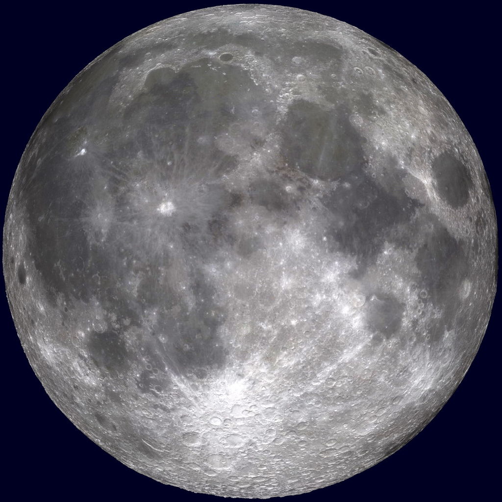
月球正面
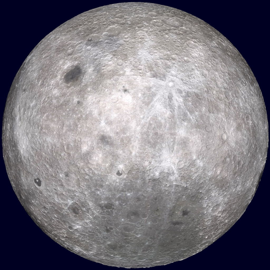
月球背面,和正面的不同之處在於缺少黑暗的月海[37]。
以及那麼多的
撞擊坑
另一個會影響月球表面地形的主要地質事件是撞擊坑[56]。小行星或彗星撞擊月球表面時都會形成隕石坑,現在估計單在月球正面直徑大於1公里的隕石坑就大約有300,000個[57],其中有些隕石坑以知名的學者、科學家、藝術家和探險家的名字命名[58]。月球地質年代是根據月面上的重大隕石撞擊事件進行分界,包括在酒海、雨海和東方海等的撞擊事件。這些撞擊事件的結構特徵是產生多層物質隆起的環,通常是由數百至數千公里直徑的圍裙狀噴發物沉積形成一個區域性的地層視界[59]。由於月球沒有大氣層、天氣變化,在最近幾十億年也沒有地質活動,大部分環形山都保存得很完好。雖然有幾個多環盆地明顯的已經很久遠,它們還是能用於分派相對的年齡。由於撞擊坑是以恆定的速率累積,計算單位面積內的撞擊坑數目可以用來估計表面的年齡[59]。阿波羅任務收集撞擊熔化的岩石以輻射測定年齡,群集在38億和41億年的年齡:這已被用來建議撞擊的後期重轟炸期[60]。
覆蓋在月球地殼上的是高度粉碎的(碎裂成更小的顆粒)和撞擊園藝下的表面層稱為風化層,是由撞擊過程形成的。最細微的風化層,是二氧化矽的月球土壤玻璃狀物體,有著像雪一樣的紋理和聞起來像用過的火藥[61]。較老的風化層表面一般比年輕的表面厚;在高地的厚度在10-20米之間,在海的厚度則是3-5米。[62] 在細緻的粉碎風化層下面是「粗風化層(megaregolith)」,厚達數公里高度碎裂的基岩[63]。
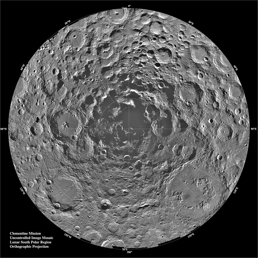
由克萊門汀號拍攝的月球南極馬賽克圖:請注意極地的永久陰影。
,不會被描述成︰替大地之母 ䷁ 蓋亞檔災殃的乎??!!
如是觀之太陽系 ䷀ 的『穩定性』,不過講其對『撞擊』之『靈敏度 』不高矣︰
假使說一個系統  很『靈敏』 sensitive ,是講當系統的『輸入』
  有一點『變化』
  ,系統之『輸出』
  ,產生很大的『改變』
  ,也就是說
,也就是說
 的『比值』很大。
然而『靈敏度』 Sensitivity 一詞,用於不同的領域、場合,常帶著點不同的意味,遇到此詞時,避免望文生義。如果將『靈敏度』用於『量測儀器』,通常是指儀表對於『輸入變化』的『分辨能力』 ,一般用著某種 之『比值』來表示。
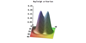
瑞利準則
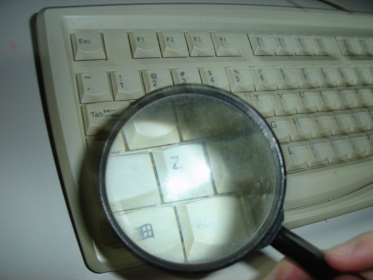
比方說 一個光學儀器的『角分辨度』 Angular resolution

表示要是透鏡和兩個物件之間的夾角少於  ,透鏡的觀察者便無法分辨出有兩個物件。不要以為『分辨能力』愈『大』,就一定是愈『好』,通常顯微鏡的放大倍數『越高』,可能操作上也『越難』 。設使每個人的『視力』都能睹『秋毫之末』,怕世間『美』『醜』的『標準』會變的吧?難想像會發明『幾 K 』的電視的哩!
『量測裝置』  是一個『物理系統』,待量測『自然萬象』
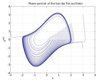
  也是一個『物理系統』,彼此『交互作用』 ── 能量和物質轉化與交換 ──,得到『度量』之數據,『測知』現象系統的『狀態』。自考察『現象』之『狀態』上來講,假使從『微觀上』將之當成由『粒子系統』所構成,或許可以用『相空間』之『相圖』來觀察︰
─── 摘自《失之豪釐,差以千里!!《中》》
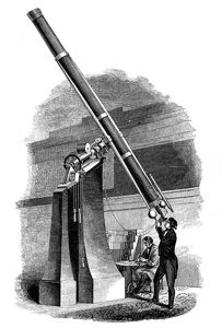
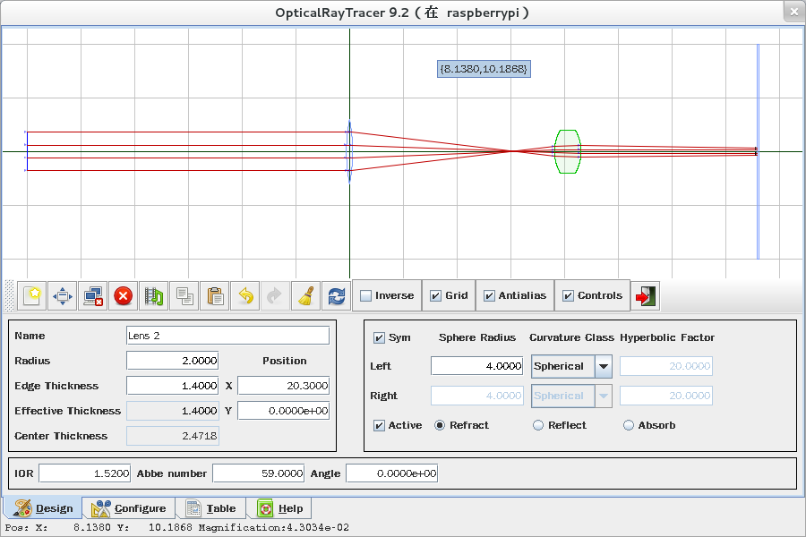
因為望遠鏡不同圖示、說明之差異︰
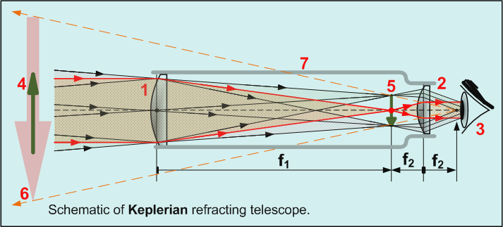
The astronomical telescope makes use of two positive lenses: the objective, which forms the image of a distant object at its focal length, and the eyepiece, which acts as a simple magnifier with which to view the image formed by the objective. Its length is equal to the sum of the focal lengths of the objective and eyepiece, and its angular magnification is -fo /fe , giving an inverted image.
 The astronomical telescope can be used for terrestrial viewing, but seeing the image upside down is a definite inconvenience. Viewing stars upside down is no problem. Another inconvenience for terrestrial viewing is the length of the astronomical telescope, equal to the sum of the focal lengths of the objective and eyepiece lenses. A shorter telescope with upright viewing is the Galilean telescope.
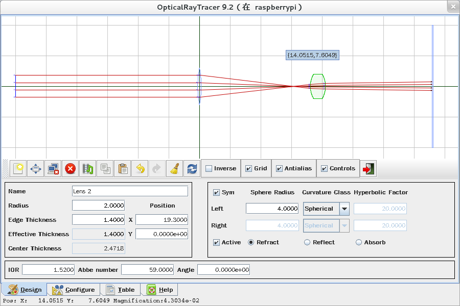
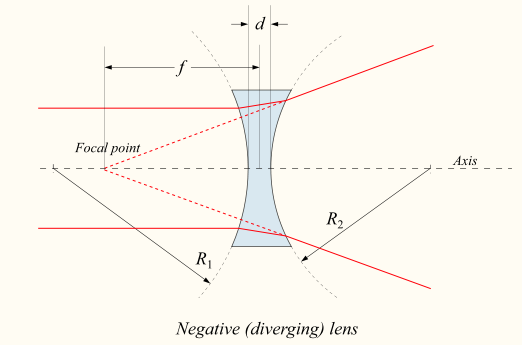
The Galilean or terrestrial telescope uses a positive objective and a negative eyepiece. It gives erect images and is shorter than the astronomical telescope with the same power. It’s angular magnification is -fo/fe .
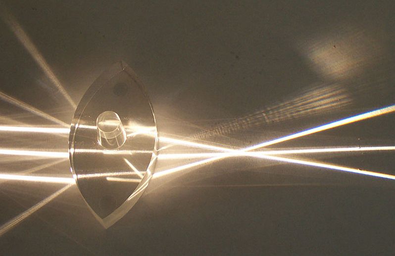
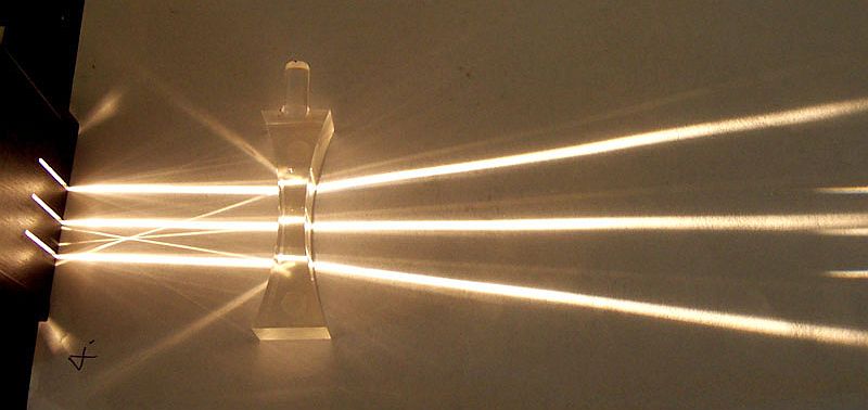
 The image below shows parallel rays from two helium-neon lasers passing through a Galilean telescope made from an objective with f=30cm and an eyepiece with f=-10cm.
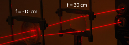 With the lenses placed 20 cm = fo+fe apart, the parallel input rays are rendered parallel again by the eyepiece lens, giving an image at infinity. This shows one of the uses of Galilean telescopes. It is useful as a collimator that takes a large beam of parallel light and reduces the size of the beam, keeping the rays parallel. The angular magnification of this Galilean telescope is 3. The beams of the helium-neon lasers were made visible with a spray can of artificial smoke.
───
 2:黃福坤(研究所)張貼:2006-10-22 13:02:58:
一旦你清楚瞭解了放大鏡的工作原理 之後要理解 望遠鏡或顯微鏡就很簡單了
放大鏡藉由將物體放在焦距內一點點 產生虛像的視角放大 讓眼睛看到更大的影像於視網膜上
若是有物體位於很遠的地方 我們知道 加上透鏡後物體會呈現於透鏡的焦點附近!
但是影像會很小 因此可以利用放大鏡的效果將其放大
若是我們在物體成像位置後放置另一個透鏡 且透鏡焦距就是該像與透鏡的距離(稍大一點)
於是 很遠處的物體所形成的像 被第二個透鏡以視角放大的方式讓我們看到 就是 望遠鏡了!
如下圖

在此假借『微擾理論』︰
Perturbation theory comprises mathematical methods for finding an approximate solution to a problem, by starting from the exact solution of a related, simpler problem. A critical feature of the technique is a middle step that breaks the problem into “solvable” and “perturbation” parts.[1] Perturbation theory is applicable if the problem at hand cannot be solved exactly, but can be formulated by adding a “small” term to the mathematical description of the exactly solvable problem.
Perturbation theory leads to an expression for the desired solution in terms of a formal power series in some “small” parameter – known as a perturbation series – that quantifies the deviation from the exactly solvable problem. The leading term in this power series is the solution of the exactly solvable problem, while further terms describe the deviation in the solution, due to the deviation from the initial problem. Formally, we have for the approximation to the full solution A, a series in the small parameter (here called ε), like the following:

In this example, A0 would be the known solution to the exactly solvable initial problem and A1, A2, … represent the higher-order terms which may be found iteratively by some systematic procedure. For small ε these higher-order terms in the series become successively smaller.
An approximate “perturbation solution” is obtained by truncating the series, usually by keeping only the first two terms, the initial solution and the “first-order” perturbation correction

………
History
Perturbation theory was first devised to solve otherwise intractable problems in the calculation of the motions of planets in the solar system. The gradually increasing accuracy of astronomical observations led to incremental demands in the accuracy of solutions to Newton’s gravitational equations, which led several notable 18th and 19th century mathematicians to extend and generalize the methods of perturbation theory. These well-developed perturbation methods were adopted and adapted to solve new problems arising during the development of Quantum Mechanics in 20th century atomic and subatomic physics.
Beginnings in the study of planetary motion
Since the planets are very remote from each other, and since their mass is small as compared to the mass of the Sun, the gravitational forces between the planets can be neglected, and the planetary motion is considered, to a first approximation, as taking place along Kepler’s orbits, which are defined by the equations of the two-body problem, the two bodies being the planet and the Sun.[3]
Since astronomic data came to be known with much greater accuracy, it became necessary to consider how the motion of a planet around the Sun is affected by other planets. This was the origin of the three-body problem; thus, in studying the system Moon–Earth–Sun the mass ratio between the Moon and the Earth was chosen as the small parameter. Lagrange and Laplace were the first to advance the view that the constants which describe the motion of a planet around the Sun are “perturbed” , as it were, by the motion of other planets and vary as a function of time; hence the name “perturbation theory” .[3]
Perturbation theory was investigated by the classical scholars — Laplace, Poisson, Gauss — as a result of which the computations could be performed with a very high accuracy. The discovery of the planet Neptune in 1848 by Urbain Le Verrier, based on the deviations in motion of the planet Uranus (he sent the coordinates to Johann Gottfried Galle who successfully observed Neptune through his telescope), represented a triumph of perturbation theory.[3]
Rise of understanding of chaotic systems
The development of basic perturbation theory for differential equations was fairly complete by the middle of the 19th century. It was at that time that Charles-Eugène Delaunay was studying the perturbative expansion for the Earth-Moon-Sun system, and discovered the so-called “problem of small denominators”.[citation needed] Here, the denominator appearing in the n-th term of the perturbative expansion could become arbitrarily small, causing the n-th correction to be as large or larger than the first-order correction.
At the turn of the 20th century, this problem led Henri Poincaré to make one of the first deductions of the existence of chaos,[citation needed] and what is poetically called the “butterfly effect”:[citation needed] that even a very small perturbation can ultimately have a very large effect on non-dissipative or “friction-free” dynamic systems.
A partial resolution of the small-divisor problem was given by the statement of the KAM theorem in 1954. Developed by Andrey Kolmogorov, Vladimir Arnold and Jürgen Moser, this theorem stated the conditions under which a system of partial differential equations will have only mildly chaotic behaviour under small perturbations.
之名舖成一番,讀者但求其實的了。
【僅供參考】
pi@raspberrypi:~ $ ipython3
Python 3.4.2 (default, Oct 19 2014, 13:31:11)
Type "copyright", "credits" or "license" for more information.

IPython 2.3.0 -- An enhanced Interactive Python.
?         -> Introduction and overview of IPython's features.
%quickref -> Quick reference.
help      -> Python's own help system.
object?   -> Details about 'object', use 'object??' for extra details.

In [1]: from sympy import *

In [2]: from sympy.physics.optics import FreeSpace, FlatRefraction, ThinLens, GeometricRay, CurvedRefraction, RayTransferMatrix

In [3]: init_printing()

In [4]: fo, ε, fe, X, I = symbols('fo, ε, fe, X, I')

In [5]: 理想模型 = ThinLens(fe) * FreeSpace(fe + fo) * ThinLens(fo)

In [6]: 理想模型
Out[6]:
⎡       fe + fo                 ⎤
⎢   1 - ───────        fe + fo  ⎥
⎢          fo                   ⎥
⎢                               ⎥
⎢      fe + fo                  ⎥
⎢  1 - ───────                  ⎥
⎢         fe     1       fe + fo⎥
⎢- ─────────── - ──  1 - ───────⎥
⎣       fo       fe         fe  ⎦

In [7]: 理想模型.A.simplify()
Out[7]:
-fe
────
 fo

In [8]: 理想模型.C.simplify()
Out[8]: 0

In [9]: 理想模型.D.simplify()
Out[9]:
-fo
────
 fe

In [10]: 理想模型 = RayTransferMatrix(-fe/fo, fe+fo, 0, -fo/fe)

In [11]: 理想模型成像 = FreeSpace(I) * 理想模型 * FreeSpace(X)

In [12]: 理想模型成像
Out[12]:
⎡-fe     I⋅fo   X⋅fe          ⎤
⎢────  - ──── - ──── + fe + fo⎥
⎢ fo      fe     fo           ⎥
⎢                             ⎥
⎢               -fo           ⎥
⎢ 0             ────          ⎥
⎣                fe           ⎦

In [13]: 理想模型成像物距 = solve(理想模型成像.B, X)

In [14]: 理想模型成像物距
Out[14]:
⎡   ⎛          2        ⎞⎤
⎢fo⋅⎝-I⋅fo + fe  + fe⋅fo⎠⎥
⎢────────────────────────⎥
⎢            2           ⎥
⎣          fe            ⎦

In [15]: 實物望遠鏡 = ThinLens(fe) * FreeSpace(fe + fo + ε) * ThinLens(fo)

In [16]: 實物望遠鏡
Out[16]:
⎡       fe + fo + ε                     ⎤
⎢   1 - ───────────        fe + fo + ε  ⎥
⎢            fo                         ⎥
⎢                                       ⎥
⎢      fe + fo + ε                      ⎥
⎢  1 - ───────────                      ⎥
⎢           fe       1       fe + fo + ε⎥
⎢- ─────────────── - ──  1 - ───────────⎥
⎣         fo         fe           fe    ⎦

In [17]: 實物望遠鏡.A.simplify()
Out[17]:
-(fe + ε)
──────────
    fo

In [18]: 實物望遠鏡.C.simplify()
Out[18]:
  ε
─────
fe⋅fo

In [19]: 實物望遠鏡.D.simplify()
Out[19]:
-(fo + ε)
──────────
    fe

In [20]: 實物望遠鏡 = RayTransferMatrix(-(fe+ε)/fo, fe+fo+ε, ε/(fe*fo), -(fo+ε)/fe)

In [21]: 誤差矩陣 = 實物望遠鏡 - 理想模型

In [22]: 誤差矩陣
Out[22]:
⎡fe   -fe - ε              ⎤
⎢── + ───────       ε      ⎥
⎢fo      fo                ⎥
⎢                          ⎥
⎢     ε        fo   -fo - ε⎥
⎢   ─────      ── + ───────⎥
⎣   fe⋅fo      fe      fe  ⎦

In [23]: 誤差矩陣.A.simplify()
Out[23]:
-ε
───
 fo

In [24]: 誤差矩陣.D.simplify()
Out[24]:
-ε
───
 fe

In [25]: 微擾矩陣 = ε * RayTransferMatrix(-1/fo, 1, 1/(fe*fo), -1/fe)

In [26]: 微擾矩陣
Out[26]:
⎡ -ε       ⎤
⎢ ───    ε ⎥
⎢  fo      ⎥
⎢          ⎥
⎢  ε    -ε ⎥
⎢─────  ───⎥
⎣fe⋅fo   fe⎦

In [27]: 微擾成像 = FreeSpace(I) * 微擾矩陣 * FreeSpace(X)

In [28]: 微擾成像
Out[28]:
⎡ I⋅ε    ε     I⋅ε     ⎛ I⋅ε    ε ⎞    ⎤
⎢───── - ──  - ─── + X⋅⎜───── - ──⎟ + ε⎥
⎢fe⋅fo   fo     fe     ⎝fe⋅fo   fo⎠    ⎥
⎢                                      ⎥
⎢    ε                X⋅ε    ε         ⎥
⎢  ─────             ───── - ──        ⎥
⎣  fe⋅fo             fe⋅fo   fe        ⎦

In [29]: solve(微擾成像.B, X)
Out[29]: [fo]

In [30]: 實物望遠鏡成像 = FreeSpace(I) * (理想模型 + 微擾矩陣) * FreeSpace(X)

In [31]: 實物望遠鏡成像
Out[31]:
⎡ I⋅ε    fe   ε     ⎛  fo   ε ⎞     ⎛ I⋅ε    fe   ε ⎞              ⎤
⎢───── - ── - ──  I⋅⎜- ── - ──⎟ + X⋅⎜───── - ── - ──⎟ + fe + fo + ε⎥
⎢fe⋅fo   fo   fo    ⎝  fe   fe⎠     ⎝fe⋅fo   fo   fo⎠              ⎥
⎢                                                                  ⎥
⎢       ε                           X⋅ε    fo   ε                  ⎥
⎢     ─────                        ───── - ── - ──                 ⎥
⎣     fe⋅fo                        fe⋅fo   fe   fe                 ⎦

In [32]: 實物望遠鏡成像物距 = solve(實物望遠鏡成像.B, X)

In [33]: 實物望遠鏡成像物距
Out[33]:
⎡   ⎛                2               ⎞⎤
⎢fo⋅⎝-I⋅fo - I⋅ε + fe  + fe⋅fo + fe⋅ε⎠⎥
⎢─────────────────────────────────────⎥
⎢                   2                 ⎥
⎣          -I⋅ε + fe  + fe⋅ε          ⎦

In [34]:


 Tutorial PowerPoint (2010 version)
 PowerPoint 97-2003 version Presentation of the Telescope Equations
 Go To Stargazing Page
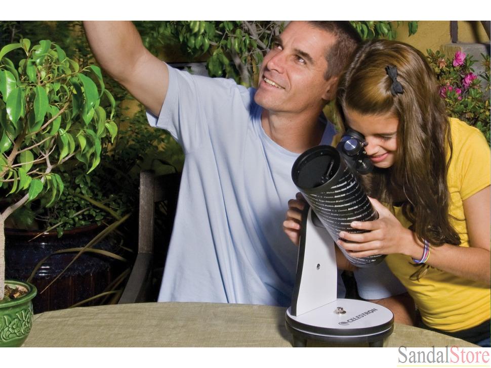
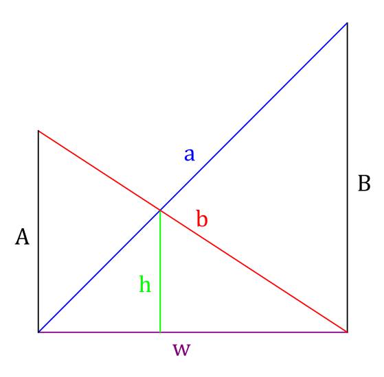
 ,你也知道它的『交叉點』距地的『高度』是
  ,那麼你能不能算出『巷寬』
  的呢?
的呢? 和
和  ,可以得到
,可以得到  與
與  。然而
。然而  ,化簡後得到
  ,這三者竟然滿足這個『不預期』之『關係式』,而且不見
  的蹤影了 。假設
  的梯子長
的梯子長  ,
, 的梯子長
的梯子長  ,由『畢氏定理』 可以得到
  與
與  ,所以
,所以  ,因此
,因此 ![{\left[ l_1^2 - l_2^2 \right]}^2 = {(h_1 + h_2)}^2 \cdot {(h_1 - h_2)}^2](http://www.freesandal.org/wp-content/ql-cache/quicklatex.com-f4939e3496dac65c89d07b3caab04b73_l3.png "Rendered by QuickLaTeX.com")
![= {(h_1 + h_2)}^2 \cdot {\left[ {(h_1 + h_2)}^2 - 4 h_1 h_2 \right] }](http://www.freesandal.org/wp-content/ql-cache/quicklatex.com-9ae577609f0e574fcd6c98b628d44ba1_l3.png "Rendered by QuickLaTeX.com") ,由於
,由於  ,將之代入上式得到
![= {(h_1 + h_2)}^2 \cdot {\left[ {(h_1 + h_2)}^2 - 4 (h_1+h_2)h \right] }](http://www.freesandal.org/wp-content/ql-cache/quicklatex.com-6cf0993fe8114e1f47673877e881fa64_l3.png "Rendered by QuickLaTeX.com")
![{\left[ l_1^2 - l_2^2 \right]}^2 = {(h_1 + h_2)}^2 \cdot {\left[ {(h_1 + h_2)}^2 - 4 (h_1+h_2)h \right] }](http://www.freesandal.org/wp-content/ql-cache/quicklatex.com-26b0991c84970e2234d7374409671e0b_l3.png "Rendered by QuickLaTeX.com")
 的『方程式』。假設
  ,如果我們定義
 ,
,

 ,果然是奇也怪哉!!
 ,那麼要怎們求出『巷寬』


 ,因此
,因此  ,因為
,因為  ,所以那個久違的『巷寬』就是
  !!
!! 與
與  來講是『對稱的』,所以除非這兩者『相等』,否則『假設』
  時,就有
時,就有  的關係存在,就可以直接求得
  的了!如此根本不需要解那個四次方程式的吧!!
 ,此時
,此時  ,那麼我們能夠求得
  之『極限值』 的嗎?因為這時
  ,因此
,因此 ,所以那個四次方程式就變成了
  ,它有四個解
  ,於是
,於是  ,由於
,由於  ,故得
,故得  。
。 與
與  不是『直角』,依然是
  。在它們是『直角』時,甚至可以得到
  ,如果將它想像成『入射角』等於『反射角』,從
  點發出的光線,將於
  點反射到
點反射到  點上。
點上。
 〒 左梯
〒 左梯  〒 右梯
〒 右梯  〒 兩梯之交叉點高
  的呢?★
的呢?★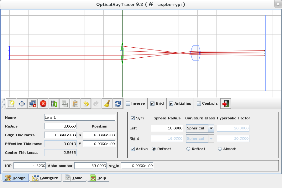

 物體,初始位置在
  ,初始速度為
  ,在
,在  軸上運動,依據牛頓的第二運動定律,它的運動滿足一個二階微分方程式︰
 的形式,比方說簡諧運動之線性彈力
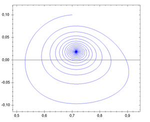
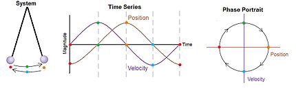
  ,微分方程式很難有『確解』,大概都得用『數值分析』的方式求解。那麼有沒有另一種運動描述辦法的呢?龐加萊和玻爾茲曼 Boltzmann 等人發展了『相空間』phase space 的想法,因為物體一旦給定了初始位置與初始速度── 一般使用動量
  ──,它的運動軌跡就由牛頓的第二運動定律所確定,相空間是一個 (位置,動量) 所構成的座標系,這樣該物體的運動軌跡就畫出了相空間裡的一條線 ── 叫做相圖 phase diagram ──。一般這條曲線不會『自相交』,因為相交代表有不同的運動軌跡可以選擇,所以一旦相交會就只能是一種『週期運動』。龐加萊在研究三體問題的相圖時,卻發現只要『初始點』── 位置或動量 ──,極微小的變化,相圖就發生很大的改變,這種『敏感性』可能導致系統的『不可預測性』或是『不穩定性』。
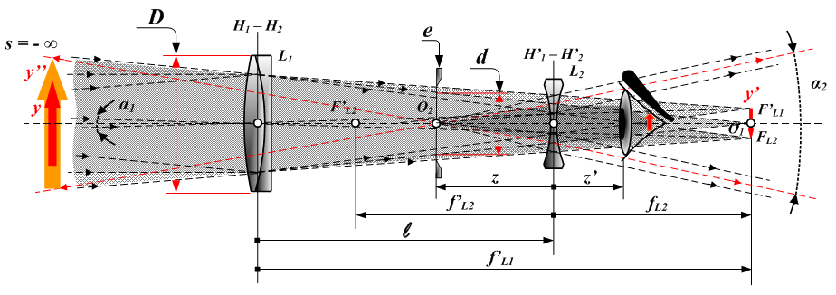
![ipython3 Python 3.4.2 (default, Oct 19 2014, 13:31:11) Type "copyright", "credits" or "license" for more information. IPython 2.3.0 -- An enhanced Interactive Python. ? -> Introduction and overview of IPython's features. %quickref -> Quick reference. help -> Python's own help system. object? -> Details about 'object', use 'object??' for extra details. In [1]: from sympy import * In [2]: from sympy.physics.optics import FreeSpace, FlatRefraction, ThinLens, GeometricRay, CurvedRefraction, RayTransferMatrix In [3]: init_printing() In [4]: do, f1, f2, z, f, e = symbols('do, f1, f2, z, f, e') In [5]: 平行光分解變換 = RayTransferMatrix(- f2/f1, f1+f2, 0, -f1/f2) In [6]: F1F2面參考系 = FreeSpace(f2) * 平行光分解變換 * FreeSpace(f1) In [7]: F1F2面參考系 Out[7]: ⎡-f₂ ⎤ ⎢──── 0 ⎥ ⎢ f₁ ⎥ ⎢ ⎥ ⎢ -f₁ ⎥ ⎢ 0 ────⎥ ⎣ f₂ ⎦ In [8]: F1F2面物距 = FreeSpace(do) In [9]: F1F2面觀看距離Z = FreeSpace(z) In [10]: 眼睛 = ThinLens(f) In [11]: 成像 = FreeSpace(e) In [12]: 光線追跡 = 成像 * 眼睛 * F1F2面觀看距離Z * F1F2面參考系 * F1F2面物距 In [13]: 光線追跡.B Out[13]: ⎛ e ⎞ ⎛ ⎛ e ⎞⎞ do⋅f₂⋅⎜- ─ + 1⎟ f₁⋅⎜e + z⋅⎜- ─ + 1⎟⎟ ⎝ f ⎠ ⎝ ⎝ f ⎠⎠ - ─────────────── - ──────────────────── f₁ f₂ In [14]: 成像條件 = solve(光線追跡.B.expand(), e) In [15]: 1 / 成像條件[0] Out[15]: 2 2 2 do⋅f₂ - f⋅f₁ + f₁ ⋅z ────────────────────── ⎛ 2 2 ⎞ f⋅⎝do⋅f₂ + f₁ ⋅z⎠ In [16]: </pre> 假設角放大率](http://www.freesandal.org/wp-content/ql-cache/quicklatex.com-5a53fa301ca64ac10958cd30508474d6_l3.png "Rendered by QuickLaTeX.com") M = \frac{f_1}{f_2}
M = \frac{f_1}{f_2} \frac{1}{e} = \frac{1}{f} - \frac{1}{\frac{d_o' - f_1}{M^2} + (z' -f_2)} }$ 。

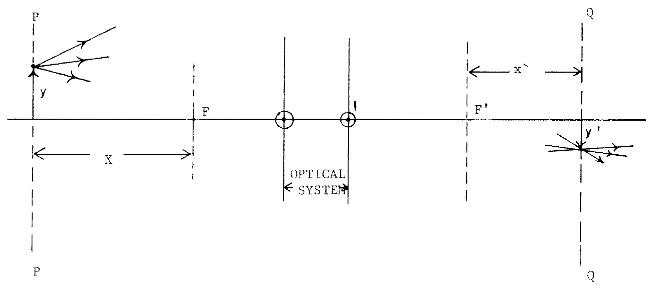

 是正或是負,
  都是正的也!如是對凸透鏡來講,無窮遠之物
  ,將成像於後焦點之平面上
  。那麼對凹透鏡來說,分明數學式子一樣!!又怎麼能一樣的呢??假使知道凹透鏡的後焦距面在凹透鏡之前,前焦距面在凹透鏡之後 ,能否釋疑呢???當真成像還是在後焦距面上!!!
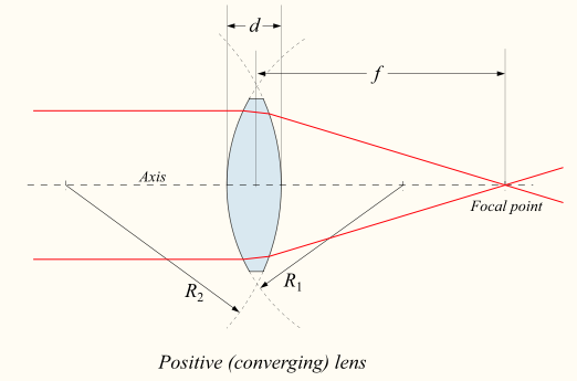


 表示物距
表示物距  表達物距
表達物距 

 的啊??倘以現象而言,同也。皆平行光罷了!!
 向凸透鏡之前焦距趨近,其像距
  ,像將在無窮遠也
  ,豈非透鏡後之平行光耶?★要是它從凸透鏡之主平面向後開始靠近前焦距面
  ,那麼
,那麼  ,難到能不是以『所見』為重,省略其透鏡後已然平行的乎!☆
 凹凸鏡面上之理耶☆