繼『大象說』之後 Michael Nielsen 接著講『過適』 overfitting 現象似乎順理成章︰

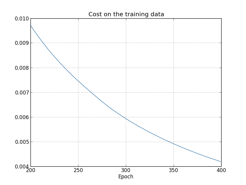
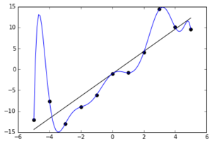
Let’s sharpen this problem up by constructing a situation where our network does a bad job generalizing to new situations. We’ll use our 30 hidden neuron network, with its 23,860 parameters. But we won’t train the network using all 50,000 MNIST training images. Instead, we’ll use just the first 1,000 training images. Using that restricted set will make the problem with generalization much more evident. We’ll train in a similar way to before, using the cross-entropy cost function, with a learning rate of and a mini-batch size of . However, we’ll train for 400 epochs, a somewhat larger number than before, because we’re not using as many training examples. Let’s use network2 to look at the way the cost function changes:

>>> import mnist_loader 
>>> training_data, validation_data, test_data = \
... mnist_loader.load_data_wrapper()
>>> import network2 
>>> net = network2.Network([784, 30, 10], cost=network2.CrossEntropyCost) 
>>> net.large_weight_initializer()
>>> net.SGD(training_data[:1000], 400, 10, 0.5, evaluation_data=test_data,
... monitor_evaluation_accuracy=True, monitor_training_cost=True)

Using the results we can plot the way the cost changes as the network learns*

*This and the next four graphs were generated by the program overfitting.py. :

This looks encouraging, showing a smooth decrease in the cost, just as we expect. Note that I’ve only shown training epochs 200 through 399. This gives us a nice up-close view of the later stages of learning, which, as we’ll see, turns out to be where the interesting action is.

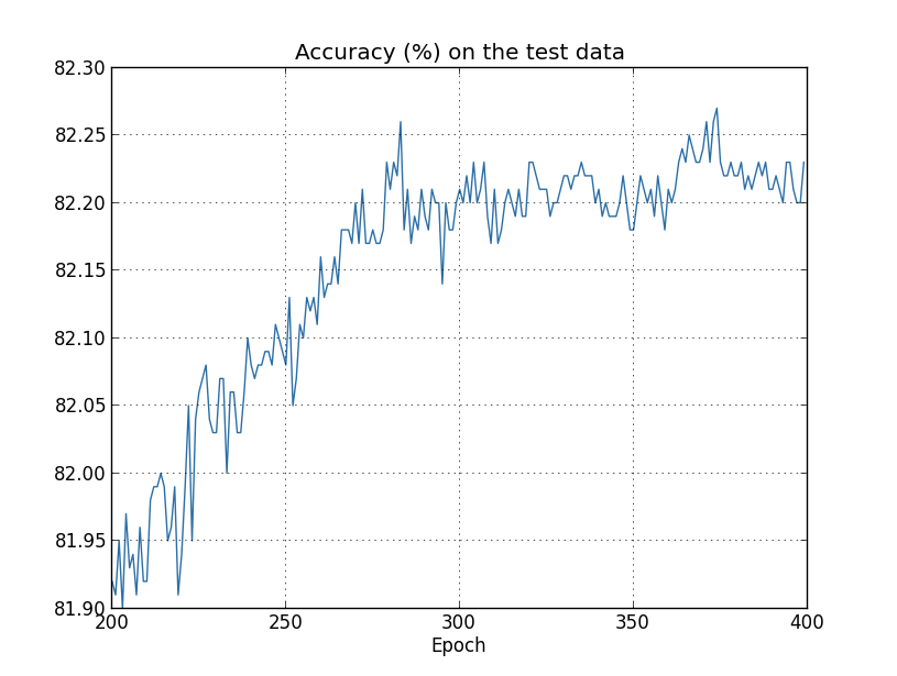
Let’s now look at how the classification accuracy on the test data changes over time:

Again, I’ve zoomed in quite a bit. In the first 200 epochs (not shown) the accuracy rises to just under 82 percent. The learning then gradually slows down. Finally, at around epoch 280 the classification accuracy pretty much stops improving. Later epochs merely see small stochastic fluctuations near the value of the accuracy at epoch 280. Contrast this with the earlier graph, where the cost associated to the training data continues to smoothly drop. If we just look at that cost, it appears that our model is still getting “better”. But the test accuracy results show the improvement is an illusion. Just like the model that Fermi disliked, what our network learns after epoch 280 no longer generalizes to the test data. And so it’s not useful learning. We say the network is overfitting or overtraining beyond epoch 280.

………

 

縱然整段文本簡易，讀來輕鬆，又以『模擬』與『圖形』來作闡釋當無疑議矣！不過讀書常貴在『不疑處有疑』！！故有『問』也？第一位吃螃蟹的人如何能下口？？

，真不知那吃 蟹的第一人，如何想來，又怎麼下得了口 ！？噗哧一笑，陡地，

  貓的理論上心頭︰

通常人們都說不要『迷信』，那『科學』自己會不會也『變成』一種迷信呢？或者說所謂的科學又是『什麼』呢？因為並非一直以來科學就是『像今天』一樣，現今的科學有著這樣的『一種精神』︰

一、事實立論
二、在事實的基礎上，建立用來解說的假設，然後形成它的理論
三、人人時時方方都可實驗，嘗試驗證或者推翻 一與二之所說
四、保持著懷疑、設想新現象、創革舊工具；再次持續不斷的想推翻一、二和三之所言。

不知這樣的精神能不能有『東』『西』之分？還是有『南』『北』之別呢？

大科學家牛頓養了一隻貓，他看到那貓因為進出門戶不方便而不『快樂』，所以在門上打了個洞，果然貓就快樂了起來。多年之後那貓生了小貓，牛頓很高興的在那個洞的旁邊又打了一個小洞，這樣小貓也一定會很『快樂』的了。真不知牛頓如何想出這個『貓的理論』︰

大貓走大洞；小貓走小洞。

難道『小貓』就不可以走『大洞』？還是不這樣『小貓』就會不『快樂』？？

，何不效法牛頓，『大』洞『小』洞『快樂』的打，一『洞』通了是『一』洞，早晚總能『洞穿』！！☿☺

─── 摘自《M♪o 之學習筆記本《辰》組元︰【䷠】黃牛之革》

 

談此『現象』的第一人又怎麼『發現』的呢？？是因為《大象說》聯想到奧卡姆之『剃刀』︰

奧卡姆剃刀（英語：Occam’s Razor, Ockham’s Razor），又稱「奧坎的剃刀」，拉丁文為lex parsimoniae，意思是簡約之法則，是由14世紀邏輯學家、聖方濟各會修士奧卡姆的威廉（William of Occam，約1287年至1347年，奧卡姆（Ockham）位於英格蘭的薩里郡） 提出的一個解決問題的法則，他在《箴言書注》2卷15題說「切勿浪費較多東西，去做『用較少的東西，同樣可以做好的事情 』。」換一種說法，如果關於同一個 問題有許多種理論，每一種都能作出同樣準確的預言，那麼應該挑選其中使用假定最少的。儘管越複雜的方法通常能作出越好的預言，但是在不考慮預言能力的情況下，前提假設越少越好。

所羅門諾夫的歸納推理理論是奧卡姆剃刀的數學公式化：^{[1][2][3][4][5][6]}在所有能夠完美描述已有觀測的可計算理論中，較短的可計算理論在估計下一次觀測結果的機率時具有較大權重。

在自然科學中，奧卡姆剃刀被作為啟發法技巧來使用，更多地作為幫助科學家發展理論模型的工具，而不是在已經發表的理論之間充當裁判角色。^[7][8]在科學方法中，奧卡姆剃刀並沒有被當做邏輯上不可辯駁的定理或者科學結論。在科學方法中對簡單性的偏好，是基於可證偽性的標準。對於某個現象的所有可接受的解釋，都存在無數個可能的、更為複雜的變體：因為你可以把任何解釋中的錯誤歸結於特例假設，從而避免該錯誤的發生。所以，較簡單的理論比複雜的理論更好，因為它們更加可檢驗。^[9][10][11]

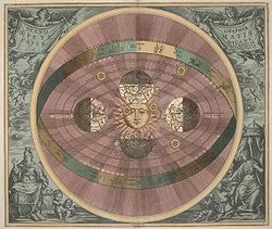
安德烈亞斯·塞拉里烏斯所繪製的哥白尼系統，見於《和諧大宇宙》（1708）。太陽、月亮和其他太陽系行星的運動既可以用地心說來解釋，也可以用日心說來解釋，都同樣有效，然而日心說只需要7個基本假設，地心說卻需要多得多的假設。在尼古拉·哥白尼的《天體運行論》序言中指出了這一點

……

數學

奧卡姆剃刀的形式之一，是基礎機率論的直接結果。根據定義，任何假設都會帶來犯錯誤機率的增加；如果一個假設不能增加理論的正確率，那麼它的唯一作用就是增加整個理論為錯誤的機率。

還有另一些從機率論理論得出奧卡姆剃刀的嘗試，包括哈羅德·傑弗里斯和埃德溫·托普森·傑納斯的著名嘗試。奧卡姆剃刀的（貝葉斯）機率基礎，是由大衛·麥克卡伊在他的著作《資訊理論、推理和學習算法》（Information Theory, Inference, and Learning Algorithms）的第28章里給出，^[30]他強調了，並不需要事先給予簡單模型一個較高的偏好值。

威廉·傑弗里斯（和哈羅德·傑弗里斯沒有關係）和詹姆斯·貝爾格爾（1991）總結和評價了原版剃刀法則中的「假設」概念。對於可能觀察到的數據來說，它是一個命題的無必要程度。^[31]他們主張：「一個可調參數較少的假設，自然地會擁有較高的後驗機率，因為它所作出的預言會更精確。^[31]他們所提出的模型，在理論的預測準確性和精確度之間尋求均衡：精確地作出正確的預言的理論，優於給出一個大的猜測範圍的或者不正確的理論。這再次反映了貝葉斯推斷中的核心概念（邊緣分布、條件機率、後驗機率）之間的聯繫 。

可能存在無必要的複雜解釋。例如，可以將矮精靈拉布列康加入任何解釋中，但是奧卡姆剃刀阻止了這樣的添加，除非它有必要

───

 

所以神通『過適』之大門耶！！

在統計學中，過適（英語：overfitting，或稱過度擬合）現象是指在調適一個統計模型時，使用過多參數。對比於可取得的資料總量來說，一個荒謬的模型只要足夠複雜，是可以完美地適應資料。過適一般可以識為違反奧卡姆剃刀原 則。當可選擇的參數的自由度超過資料所包含資訊內容時，這會導致最後（調適後）模型使用任意的參數，這會減少或破壞模型一般化的能力更甚於適應資料。過適 的可能性不只取決於參數個數和資料，也跟模型架構與資料的一致性有關。此外對比於資料中預期的雜訊或錯誤數量，跟模型錯誤的數量也有關。

過適現象的觀念對機器學習也是很重要的。通常一個學習演算法是藉由訓練範例來訓練的。亦即預期結果的範例是可知的。而學習者則被認為須達到可以預測出其它範例的正確的結果，因此，應適用於一般化的情況而非只是訓練時所使用的現有資料（根據它的歸納偏向）。然而，學習者卻會去適應訓練資料中太特化但又隨機的特徵，特別是在當學習過程太久或範例太少時。在過適的過程中，當預測訓練範例結果的表現增加時，應用在未知資料的表現則變更差 。

在統計和機器學習中，為了避免過適現象，須要使用額外的技巧（如交叉驗證、early stopping、貝斯信息量準則、赤池信息量準則或model comparison），以指出何時會有更多訓練而沒有導致更好的一般化。人工神經網路的過適過程亦被認知為過度訓練（英語： overtraining）。在treatmeant learning中，使用最小最佳支援值（英語：minimum best support value）來避免過適。

相對於過適是指，使用過多參數，以致太適應資料而非一般情況，另一種常見的現象是使用太少參數，以致於不適應資料，這則稱為乏適（英語：underfitting，或稱：擬合不足）現象。

───

Noisy (roughly linear) data is fitted to both linear and polynomial functions. Although the polynomial function is a perfect fit, the linear version can be expected to generalize better. In other words, if the two functions were used to extrapolate the data beyond the fit data, the linear function would make better predictions.

……

Machine learning

Usually a learning algorithm is trained using some set of “training data”: exemplary situations for which the desired output is known. The goal is that the algorithm will also perform well on predicting the output when fed “validation data” that was not encountered during its training.

Overfitting is the use of models or procedures that violate Occam’s razor, for example by including more adjustable parameters than are ultimately optimal, or by using a more complicated approach than is ultimately optimal. For an example where there are too many adjustable parameters, consider a dataset where training data for y can be adequately predicted by a linear function of two dependent variables. Such a function requires only three parameters (the intercept and two slopes). Replacing this simple function with a new, more complex quadratic function, or with a new, more complex linear function on more than two dependent variables, carries a risk: Occam’s razor implies that any given complex function is a priori less probable than any given simple function. If the new, more complicated function is selected instead of the simple function, and if there was not a large enough gain in training-data fit to offset the complexity increase, then the new complex function “overfits” the data, and the complex overfitted function will likely perform worse than the simpler function on validation data outside the training dataset, even though the complex function performed as well, or perhaps even better, on the training dataset.^[2]

When comparing different types of models, complexity cannot be measured solely by counting how many parameters exist in each model; the expressivity of each parameter must be considered as well. For example, it is nontrivial to directly compare the complexity of a neural net (which can track curvilinear relationships) with m parameters to a regression model with n parameters.^[2]

Overfitting is especially likely in cases where learning was performed too long or where training examples are rare, causing the learner to adjust to very specific random features of the training data, that have no causal relation to the target function. In this process of overfitting, the performance on the training examples still increases while the performance on unseen data becomes worse.

As a simple example, consider a database of retail purchases that includes the item bought, the purchaser, and the date and time of purchase. It’s easy to construct a model that will fit the training set perfectly by using the date and time of purchase to predict the other attributes; but this model will not generalize at all to new data, because those past times will never occur again.

Generally, a learning algorithm is said to overfit relative to a simpler one if it is more accurate in fitting known data (hindsight) but less accurate in predicting new data (foresight). One can intuitively understand overfitting from the fact that information from all past experience can be divided into two groups: information that is relevant for the future and irrelevant information (“noise”). Everything else being equal, the more difficult a criterion is to predict (i.e., the higher its uncertainty), the more noise exists in past information that needs to be ignored. The problem is determining which part to ignore. A learning algorithm that can reduce the chance of fitting noise is called robust.

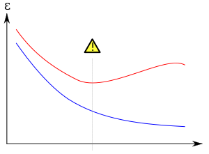
Overfitting/overtraining in supervised learning (e.g., neural network). Training error is shown in blue, validation error in red, both as a function of the number of training cycles. If the validation error increases(positive slope) while the training error steadily decreases(negative slope) then a situation of overfitting may have occurred. The best predictive and fitted model would be where the validation error has its global minimum.

───

 

總需知『以偏概全』 是誤謬，『以全蓋偏』易犯『區群謬誤』也︰

區群謬誤（Ecological fallacy），又稱生態謬誤，層次謬誤，是一種在分析統計資料時常犯的錯誤。和以偏概全相反，區群謬誤是一種以全概偏，如果僅基於群體的統計數據就對其下屬的個體性質作出推論，就是犯上區群謬誤。這謬誤假設了群體中的所有個體都有群體的性質（因此塑型（Sterotypes）也可能犯上區群謬誤）。區群謬誤的相反情況為化約主義（Reductionism)。

起源

Ecological fallacy這名詞最先見於William S. Robinson在1950年的文章^[1]。在1930年美國人口普查結果中，Robinson分析了48個州的識字率以及新移民人 口比例的關係。他發現兩者之間的相關係數為0.53，即代表若一個州的新移民比率愈高，平均來說這個州的識字率便愈高。但當分析個體資料時，便發現相關係 數便是-0.11，即平均來說新移民比本地人的識字率低。出現這種看似矛盾的結果，其實是因為新移民都傾向在識字率較高的州份定居。Robinson因此 提出在處理群體資料，或區群資料時，必須注意到資料對個體的適用性。

這並非指任何以群體資料對個體性質作出的推論都是錯誤的，但在推論時必須注意群體資料會否把群體內的變異隱藏起來。

───

 

『刻板印象』導致過度簡化之情事，奈何廣告卻愛用的呢？不管『夢露之裙』或『 鉤足之吻』純是老梗之 stereotype 乎！

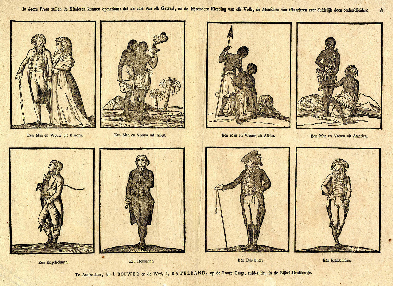
一張十八世紀時荷蘭的圖畫，裡頭將亞洲、美洲及非洲的人描述成野蠻人，下方呈現的則分別是英國人、荷蘭人、德國人和法國人。

 

明眼者能不謹慎耶？？？