一段平鋪直敘之文章，寫得清楚容易了解︰

Learning rate: Suppose we run three MNIST networks with three different learning rates, $\eta = 0.025$ $η = 0.025$ , $\eta = 0.25$ $η = 0.25$ and $\eta = 2.5$ $η = 2.5$ , respectively. We’ll set the other hyper-parameters as for the experiments in earlier sections, running over 30 epochs, with a mini-batch size of 10, and with $\lambda = 5.0$ $λ = 5.0$ . We’ll also return to using the full $50, 000$ training images. Here’s a graph showing the behaviour of the training cost as we train*

*The graph was generated by multiple_eta.py.:

With $\eta = 0.025$

η = 0.025

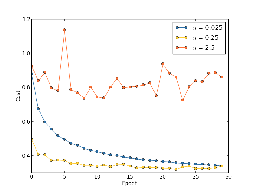the cost decreases smoothly until the final epoch. With $\eta = 0.25$

η = 0.25

the cost initially decreases, but after about

20

epochs it is near saturation, and thereafter most of the changes are merely small and apparently random oscillations. Finally, with $\eta =2.5$

η = 2.5

the cost makes large oscillations right from the start. To understand the reason for the oscillations, recall that stochastic gradient descent is supposed to step us gradually down into a valley of the cost function,

However, if $\eta$

η

is too large then the steps will be so large that they may actually overshoot the minimum, causing the algorithm to climb up out of the valley instead. That’s likely*

*This picture is helpful, but it’s intended as an intuition-building illustration of what may go on, not as a complete, exhaustive explanation. Briefly, a more complete explanation is as follows: gradient descent uses a first-order approximation to the cost function as a guide to how to decrease the cost. For large $η$ , higher-order terms in the cost function become more important, and may dominate the behaviour, causing gradient descent to break down. This is especially likely as we approach minima and quasi-minima of the cost function, since near such points the gradient becomes small, making it easier for higher-order terms to dominate behaviour.

what’s causing the cost to oscillate when $\eta =2.5$ $η = 2.5$ . When we choose $\eta = 0.25$ $η = 0.25$ the initial steps do take us toward a minimum of the cost function, and it’s only once we get near that minimum that we start to suffer from the overshooting problem. And when we choose $\eta = 0.025$ $η = 0.025$ we don’t suffer from this problem at all during the first $30$ epochs. Of course, choosing $η$ so small creates another problem, namely, that it slows down stochastic gradient descent. An even better approach would be to start with $\eta = 0.25$ $η = 0.25$ , train for $20$ epochs, and then switch to $\eta = 0.025$ $η = 0.025$ . We’ll discuss such variable learning rate schedules later. For now, though, let’s stick to figuring out how to find a single good value for the learning rate, $\eta$ $η$ .

With this picture in mind, we can set $\eta$ $η$ as follows. First, we estimate the threshold value for $\eta$ $η$ at which the cost on the training data immediately begins decreasing, instead of oscillating or increasing. This estimate doesn’t need to be too accurate. You can estimate the order of magnitude by starting with $\eta = 0.01$ $η = 0.01$ . If the cost decreases during the first few epochs, then you should successively try $\eta = 0.1, 1.0, \ldots$ $η = 0.1, 1.0, \dots$ until you find a value for $\eta$ $η$ where the cost oscillates or increases during the first few epochs. Alternately, if the cost oscillates or increases during the first few epochs when $\eta = 0.01$ $η = 0.01$ , then try $\eta = 0.001, 0.0001, \ldots$ $η = 0.001, 0.0001, \dots$ until you find a value for $\eta$ $η$ where the cost decreases during the first few epochs. Following this procedure will give us an order of magnitude estimate for the threshold value of $\eta$ $η$ . You may optionally refine your estimate, to pick out the largest value of $\eta$ $η$ at which the cost decreases during the first few epochs, say $\eta = 0.5$ $η = 0.5$ or $\eta = 0.2$ $η = 0.2$ (there’s no need for this to be super-accurate). This gives us an estimate for the threshold value of $\eta$ $η$ .

Obviously, the actual value of $\eta$ $η$ that you use should be no larger than the threshold value. In fact, if the value of $\eta$ $η$ is to remain usable over many epochs then you likely want to use a value for $\eta$ $η$ that is smaller, say, a factor of two below the threshold. Such a choice will typically allow you to train for many epochs, without causing too much of a slowdown in learning.

In the case of the MNIST data, following this strategy leads to an estimate of $0.1$ for the order of magnitude of the threshold value of $\eta$ $η$ . After some more refinement, we obtain a threshold value $\eta = 0.5$ $η = 0.5$ . Following the prescription above, this suggests using $\eta = 0.25$ $η = 0.25$ as our value for the learning rate. In fact, I found that using $\eta = 0.5$ $η = 0.5$ worked well enough over $30$ epochs that for the most part I didn’t worry about using a lower value of $\eta$ $η$ .

This all seems quite straightforward. However, using the training cost to pick $\eta$ $η$ appears to contradict what I said earlier in this section, namely, that we’d pick hyper-parameters by evaluating performance using our held-out validation data. In fact, we’ll use validation accuracy to pick the regularization hyper-parameter, the mini-batch size, and network parameters such as the number of layers and hidden neurons, and so on. Why do things differently for the learning rate? Frankly, this choice is my personal aesthetic preference, and is perhaps somewhat idiosyncratic. The reasoning is that the other hyper-parameters are intended to improve the final classification accuracy on the test set, and so it makes sense to select them on the basis of validation accuracy. However, the learning rate is only incidentally meant to impact the final classification accuracy. Its primary purpose is really to control the step size in gradient descent, and monitoring the training cost is the best way to detect if the step size is too big. With that said, this is a personal aesthetic preference. Early on during learning the training cost usually only decreases if the validation accuracy improves, and so in practice it’s unlikely to make much difference which criterion you use.

───

原本無需註釋，只因『美學偏好』 aesthetic preference 一語，幾句陳述啟人疑竇。比方『剃刀原理』喜歡『簡明理論』，可說是科學之『美學原則』。歐式幾何學從點、線、面等等『基本概念』，藉著五大『公設』，推演整部幾何學，實起現今『公設法』之先河，可說是一種『美學』的『論述典範』。如是『超參數』居處『神經網絡』之先，必先擇取『破題』方能確立某一『神經網絡模型』，自當是以『驗證正確率』為依歸。不過這『學習率』Learning rate 卻是根植於『梯度下降法』方法論的『內廩參數』，故有此一分說的耶？或許 Michael Nielsen 先生暗指科學上還有一以『邏輯先後』為理據之傳統的乎！好比︰

乾坤萬象自有它之內蘊機理，好似程序能將系統的輸入轉成輸出，或許這正是科學所追求之『萬物理論』的吧？？

生︰西方英國有學者，名作『史蒂芬‧沃爾夫勒姆』 Stephen Wolfram 創造『 Mathematica 』，曾寫

《一種新科學》 A New Kind of Science

，分類『細胞自動機』，欲究事物之本原。

Cellular automaton

A cellular automaton (pl. cellular automata, abbrev. CA) is a discrete model studied in computability theory, mathematics, physics, complexity science, theoretical biology and microstructure modeling. Cellular automata are also called cellular spaces, tessellation automata, homogeneous structures, cellular structures, tessellation structures, and iterative arrays.^[2]

A cellular automaton consists of a regular grid of cells, each in one of a finite number of states, such as on and off (in contrast to a coupled map lattice). The grid can be in any finite number of dimensions. For each cell, a set of cells called its neighborhood is defined relative to the specified cell. An initial state (time t = 0) is selected by assigning a state for each cell. A new generation is created (advancing t by 1), according to some fixed rule (generally, a mathematical function) that determines the new state of each cell in terms of the current state of the cell and the states of the cells in its neighborhood. Typically, the rule for updating the state of cells is the same for each cell and does not change over time, and is applied to the whole grid simultaneously, though exceptions are known, such as the stochastic cellular automaton and asynchronous cellular automaton.

─── 摘自《M♪o 之學習筆記本《辰》組元︰【䷀】萬象一原》

如果緣起性空，本原何來？萬象何起？？既然一切還原於『原子』！！

還原論

還原論或還原主義（英語：Reductionism，又譯化約論），是一種哲學思想，認為複雜的系統、事務、現象可以通過將其化解為各部分之組合的方法，加以理解和描述。

還原論的思想在自然科學中有很大影響，例如認為化學是以物理學為基礎，生物學是以化學為基礎，等等。在社會科學中，圍繞還原論的觀點有很大爭議，例如心理學是否能夠歸結於生物學，社會學是否能歸結於心理學，政治學能否歸結於社會學，等等。

───

Reductionism

Reductionism refers to several related but different philosophical positions regarding the connections between phenomena, or theories, “reducing” one to another, usually considered “simpler” or more “basic”.^[1] The Oxford Companion to Philosophy suggests that it is “one of the most used and abused terms in the philosophical lexicon” and suggests a three part division:^[2]

Ontological reductionism: a belief that the whole of reality consists of a minimal number of parts
Methodological reductionism: the scientific attempt to provide explanation in terms of ever smaller entities
Theory reductionism: the suggestion that a newer theory does not replace or absorb the old, but reduces it to more basic terms. Theory reduction itself is divisible into three: translation, derivation and explanation.^[3]

Reductionism can be applied to objects, phenomena, explanations, theories, and meanings.^[3]^[4]^[5]

In the sciences, application of methodological reductionism attempts explanation of entire systems in terms of their individual, constituent parts and their interactions. Thomas Nagel speaks of psychophysical reductionism (the attempted reduction of psychological phenomena to physics and chemistry), as do others and physico-chemical reductionism (the attempted reduction of biology to physics and chemistry), again as do others.^[6] In a very simplified and sometimes contested form, such reductionism is said to imply that a system is nothing but the sum of its parts.^[4]^[7] However, a more nuanced view is that a system is composed entirely of its parts, but the system will have features that none of the parts have.^[8] “The point of mechanistic explanations is usually showing how the higher level features arise from the parts.”^[7]

Other definitions are used by other authors. For example, what Polkinghorne calls conceptual or epistemological reductionism^[4] is the definition provided by Blackburn^[9] and by Kim:^[10] that form of reductionism concerning a program of replacing the facts or entities entering statements claimed to be true in one area of discourse with other facts or entities from another area, thereby providing a relationship between them. Such a connection is provided where the same idea can be expressed by “levels” of explanation, with higher levels reducible if need be to lower levels. This use of levels of understanding in part expresses our human limitations in grasping a lot of detail. However, “most philosophers would insist that our role in conceptualizing reality [our need for an hierarchy of “levels” of understanding] does not change the fact that different levels of organization in reality do have different properties.”^[8]

As this introduction suggests, there are a variety of forms of reductionism, discussed in more detail in subsections below.

Reductionism strongly reflects a certain perspective on causality. In a reductionist framework, the phenomena that can be explained completely in terms of relations between other more fundamental phenomena, are called epiphenomena. Often there is an implication that the epiphenomenon exerts no causal agency on the fundamental phenomena that explain it. The epiphenomena are sometimes said to be “nothing but” the outcome of the workings of the fundamental phenomena, although the epiphenomena might be more clearly and efficiently described in very different terms. There is a tendency to avoid taking an epiphenomenon as being important in its own right. This attitude may extend to cases where the fundamentals are not clearly able to explain the epiphenomena, but are expected to by the speaker. In this way, for example, morality can be deemed to be “nothing but” evolutionary adaptation, and consciousness can be considered “nothing but” the outcome of neurobiological processes.

Reductionism does not preclude the existence of what might be called emergent phenomena, but it does imply the ability to understand those phenomena completely in terms of the processes from which they are composed. This reductionist understanding is very different from emergentism, which intends that what emerges in “emergence” is more than the sum of the processes from which it emerges.^[11]

Duck_of_Vaucanson

Descartes held that non-human animals could be reductively explained as automata — De homine, 1662.

───

焉有

夸克

夸克（英語：quark，又譯「層子」或「虧子」）是一種基本粒子，也是構成物質的基本單元。夸克互相結合，形成一種複合粒子，叫強子，強子中最穩定的是質子和中子，它們是構成原子核的單元^[1]。由於一種叫「夸克禁閉」的現象，夸克不能夠直接被觀測到，或是被分離出來；只能夠在強子裏面找到夸克^[2]^[3]。就是因為這個原因，我們對夸克的所知大都是來自對強子的觀測。

我們知道夸克有六種，夸克的種類被稱為「味」，它們是上、下、魅、奇、底及頂^[4]。上及下夸克的質量是所有夸克中最低的。較重的夸克會通過一個叫粒子衰變的過程，來迅速地變成上或下夸克。粒子衰變是一個從高質量態變成低質量態的過程。就是因為這個原因，上及下夸克一般來說很穩定，所以它們在宇宙中很常見，而奇、魅、頂及底則只能經由高能粒子的碰撞產生（例如宇宙射線及粒子加速器）。

夸克有著多種不同的內在特性，包括電荷、色荷、自旋及質量等。在標準模型中，夸克是唯一一種能經受全部四種基本交互作用的基本粒子，基本交互作用有時會被稱為「基本力」（電磁、重力、強交互作用及弱交互作用）。夸克同時是現時已知唯一一種基本電荷非整數的粒子。夸克每一種味都有一種對應的反粒子，叫反夸克，它跟夸克的不同之處，只在於它的一些特性跟夸克大小一樣但正負不同。

夸克模型分別由默里·蓋爾曼與喬治·茨威格於1964年獨立地提出^[5]。引入夸克這一概念，是為了能更好地整理各種強子，而當時並沒有甚麼能證實夸克存在的物理證據，直到1968年SLAC開發出深度非彈性散射實驗為止^[6]^[7]。夸克的六種味已經全部被加速器實驗所觀測到；而於1995年在費米實驗室被觀測到的頂夸克，是最後發現的一種^[5]。

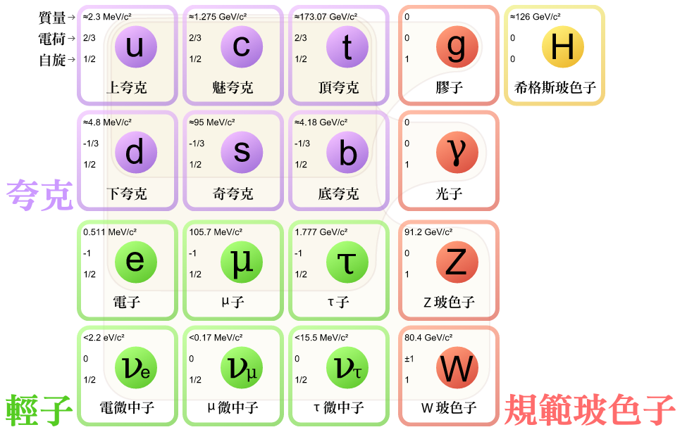
Standard_Model_of_Elementary_Particles_zh-hant

標準模型中的粒子有六種是夸克（圖中用紫色表示）。左邊的三行中，每一行構成物質的一代。

───

耶！！豈是梯度下降法之數學以及歷史淵源

‧ Gradient descent

‧ Euler method

不足以解釋『學習率』 $\eta$ 何指的乎？？終究還是得回歸『解析』或『數值計算』之審思明辨的吧！！？？

Stiff equation

In mathematics, a stiff equation is a differential equation for which certain numerical methods for solving the equation are numerically unstable, unless the step size is taken to be extremely small. It has proven difficult to formulate a precise definition of stiffness, but the main idea is that the equation includes some terms that can lead to rapid variation in the solution.

When integrating a differential equation numerically, one would expect the requisite step size to be relatively small in a region where the solution curve displays much variation and to be relatively large where the solution curve straightens out to approach a line with slope nearly zero. For some problems this is not the case. Sometimes the step size is forced down to an unacceptably small level in a region where the solution curve is very smooth. The phenomenon being exhibited here is known as stiffness. In some cases we may have two different problems with the same solution, yet problem one is not stiff and problem two is stiff. Clearly the phenomenon cannot be a property of the exact solution, since this is the same for both problems, and must be a property of the differential system itself. It is thus appropriate to speak of stiff systems.

Motivating example

Consider the initial value problem

\,y'(t)=-15y(t),\quad t\geq 0,y(0)=1.

(1)

The exact solution (shown in cyan) is

y(t)=e^{-15t}\,

with

y(t)\to 0

t\to \infty .

(2)

We seek a numerical solution that exhibits the same behavior.

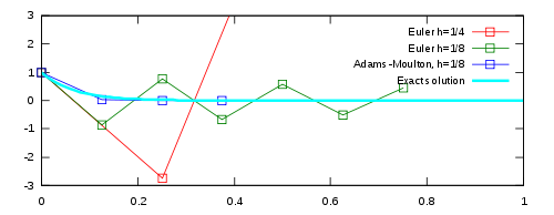
The figure (right) illustrates the numerical issues for various numerical integrators applied on the equation.

Euler’s method with a step size of h = 1/4 oscillates wildly and quickly exits the range of the graph (shown in red).
Euler’s method with half the step size, h = 1/8, produces a solution within the graph boundaries, but oscillates about zero (shown in green).
The trapezoidal method (that is, the two-stage Adams–Moulton method) is given by

$y_{n+1}=y_{n}+{\frac {1}{2}}h\left(f(t_{n},y_{n})+f(t_{n+1},y_{n+1})\right),$ (3)

where y ′ = f ( t , y ) $\textstyle y'=f(t,y)$ . Applying this method instead of Euler’s method gives a much better result (blue). The numerical results decrease monotonically to zero, just as the exact solution does.

One of the most prominent examples of the stiff ODEs is a system that describes the chemical reaction of Robertson:

{\dot {x}}=-0.04x+10^{4}y\cdot z

{\dot {y}}=0.04x-10^{4}y\cdot z-3\cdot 10^{7}y^{2}

{\dot {z}}=3\cdot 10^{7}y^{2}

(4)

If one treats this system on a short interval, for example, t ∈ [ 0 , 40 ] {\displaystyle t\in [0,40]} $t\in [0,40]$ there is no problem in numerical integration. However, if the interval is very large (10¹¹ say), then many standard codes fail to integrate it correctly.

Additional examples are the sets of ODEs resulting from the temporal integration of large chemical reaction mechanisms. Here, the stiffness arises from the coexistence of very slow and very fast reactions. To solve them, the software packages KPP and Autochem can be used.

Explicit numerical methods exhibiting instability when integrating a stiff ordinary differential equation

日	一	二	三	四	五	六
« 5 月				7 月 »
			1	2	3	4
5	6	7	8	9	10	11
12	13	14	15	16	17	18
19	20	21	22	23	24	25
26	27	28	29	30

FreeSandal

每日彙整: 2016-06-18

W!o+ 的《小伶鼬工坊演義》︰神經網絡【超參數評估】三

Cellular automaton

還原論

Reductionism

夸克

Stiff equation

Motivating example

輕。鬆。學。部落客