『暗室裡抓黑貓』者最好先確定那貓是『存在』的吧！

存在性定理

在數學中，存在性定理是一類以「存在……」開頭的定理的總稱。有時前面也會加上一些限定，比如說「對於所有的……，存在 ……」。形式上來說，存在性定理是指在定理的命題敘述中涉及存在量詞的定理。實際中，許多存在性定理並不會明確地用到「存在」這個字眼，比如說「正弦函數是連續的。」這個定理中並沒有出現「存在」一詞，但仍是一個存在性定理。因為「連續性」的定義是一個存在性的定義。

二十世紀初期曾經有過關於純粹的存在性定理的爭論。在數學結構主義的角度上，如果承認此種定理的存在，那麼數學的實用性將會降低。而與之相反的觀點認為抽象的手段可以達到數值分析所無法達到的目的。

……

‘Pure’ existence results

An existence theorem is purely theoretical if the proof given of it doesn’t also indicate a construction of whatever kind of object the existence of which is asserted. Such a proof is non-constructive, and the point is that the whole approach may not lend itself to construction.^[2] In terms of algorithms, purely theoretical existence theorems bypass all algorithms for finding what is asserted to exist. They contrast with “constructive” existence theorems.^[3] Many constructivist mathematicians work in extended logics (such as intuitionistic logic) where such existence statements are intrinsically weaker than their constructive counterparts.

Such purely theoretical existence results are in any case ubiquitous in contemporary mathematics. For example, John Nash‘s original proof of the existence of a Nash equilibrium, from 1951, was such an existence theorem. In 1962 a constructive approach was found.^[4]

───

因此欲作『最佳化』計算者，豈可不考究解之『適切性』的呢？

最佳化

最佳化，是應用數學的一個分支，主要研究以下形式的問題：

數學表述

主要研究以下形式的問題：

給定一個函數

f:A\to \mathbb {R}

，尋找一個元素

\mathbf {x} ^{0}\in A

使得對於所有

A

中的

\mathbf {x}

，

f(\mathbf {x} ^{0})\leq f(\mathbf {x} )

（最小化）；或者

f(\mathbf {x} ^{0})\geq f(\mathbf {x} )

（最大化）。

這類定式有時還稱為「數學規劃」（譬如，線性規劃）。許多現實和理論問題都可以建模成這樣的一般性框架。

典型的， $A$ 一般為歐幾里得空間 $\mathbb {R} ^{n}$ 中的子集，通常由一個 $A$ 必須滿足的約束等式或者不等式來規定。 $A$ 的元素被稱為是可行解。函數 $f$ 被稱為目標函數，或者代價函數。一個最小化（或者最大化）目標函數的可行解被稱為最優解。

一般情況下，會存在若干個局部的極小值或者極大值。局部極小值 $x^{*}$ 定義為對於一些 $\delta >0$ ，以及所有的 $x$ 滿足

\|\mathbf {x} -\mathbf {x} ^{*}\|\leq \delta

;

公式

f(\mathbf {x} ^{*})\leq f(\mathbf {x} )

成立。這就是說，在 $\mathbf {x} ^{*}$ 周圍的一些閉球上，所有的函數值都大於或者等於在該點的函數值。一般的，求局部極小值是容易的，但是要確保其為全域性的最小值，則需要一些附加性的條件，例如，該函數必須是凸函數。

符號表示

最佳化問題通常有一些較特別的符號標示方法。例如：

\mathrm {min} _{x\in \mathbb {R} }\;x^{2}+1

這是要求表達式 $x^{2}+1$ 的最小值，這裡x取值為全體實數， $\mathbb {R}$ 。這個問題的最小值應該是 $1$ ，當 $x=0$ 。

\mathrm {max} _{x\in \mathbb {R} }\;2x

這是要求表達式 $2x$ 的最大值，同樣地， $x$ 在全體實數上取值。對於這個問題，由於該表達式不是有上界的，因此不存在最大值，因此，答案應該是無限大，或者是不可定義的。

\operatorname {argmin} _{x\in [-\infty ;-1]}\;x^{2}+1\,

這是求使表達式x²+1 達到最小值時x的值。在這裡x被限定在區間[-∞ ,-1]之間，所以上式的值是-1。

───

此之所以 Michael Nielsen 先生這裡用

『知之為知之』、『不知為不知』是知也的精神

泛談『其它』人工神經元之『模型』︰

Other models of artificial neuron

Up to now we’ve built our neural networks using sigmoid neurons. In principle, a network built from sigmoid neurons can compute any function. In practice, however, networks built using other model neurons sometimes outperform sigmoid networks. Depending on the application, networks based on such alternate models may learn faster, generalize better to test data, or perhaps do both. Let me mention a couple of alternate model neurons, to give you the flavor of some variations in common use.

Perhaps the simplest variation is the tanh (pronounced “tanch”) neuron, which replaces the sigmoid function by the hyperbolic tangent function. The output of a tanh neuron with input $x$ , weight vector $w$ $w$ , and bias $b$ $b$ is given by

\tanh(w \cdot x+b), \ \ \ \ (109)

where $\tanh$ is, of course, the hyperbolic tangent function. It turns out that this is very closely related to the sigmoid neuron. To see this, recall that the $\tanh$ function is defined by

\tanh(z) \equiv \frac{e^z-e^{-z}}{e^z+e^{-z}}. \ \ \ \ (110)

With a little algebra it can easily be verified that

\sigma(z) = \frac{1+\tanh(z/2)}{2}, \ \ \ \ (111)

that is, $\tanh$ is just a rescaled version of the sigmoid function. We can also see graphically that the $\tanh$ function has the same shape as the sigmoid function,

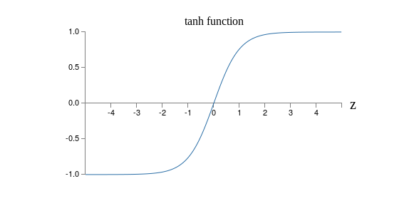
One difference between tanh neurons and sigmoid neurons is that the output from tanh neurons ranges from -1 to 1, not 0 to 1. This means that if you’re going to build a network based on tanh neurons you may need to normalize your outputs (and, depending on the details of the application, possibly your inputs) a little differently than in sigmoid networks.

Similar to sigmoid neurons, a network of tanh neurons can, in principle, compute any function*

*There are some technical caveats to this statement for both tanh and sigmoid neurons, as well as for the rectified linear neurons discussed below. However, informally it’s usually fine to think of neural networks as being able to approximate any function to arbitrary accuracy.

mapping inputs to the range -1 to 1. Furthermore, ideas such as backpropagation and stochastic gradient descent are as easily applied to a network of tanh neurons as to a network of sigmoid neurons.

Exercise

Prove the identity in Equation (111).

Which type of neuron should you use in your networks, the tanh or sigmoid? A priori the answer is not obvious, to put it mildly! However, there are theoretical arguments and some empirical evidence to suggest that the tanh sometimes performs better*

*See, for example, Efficient BackProp, by Yann LeCun, Léon Bottou, Genevieve Orr and Klaus-Robert Müller (1998), and Understanding the difficulty of training deep feedforward networks, by Xavier Glorot and Yoshua Bengio (2010).

. Let me briefly give you the flavor of one of the theoretical arguments for tanh neurons. Suppose we’re using sigmoid neurons, so all activations in our network are positive. Let’s consider the weights $w^{l+1}_{jk}$ $w_{j k}^{l + 1}$ input to the $j$ th neuron in the $l +1$ $l + 1$ th layer. The rules for backpropagation (see here) tell us that the associated gradient will be $a^l_k \delta^{l+1}_j$ $a_{k}^{l} δ_{j}^{l + 1}$ . Because the activations are positive the sign of this gradient will be the same as the sign of $\delta^{l+1}_j$ $δ_{j}^{l + 1}$ . What this means is that if $\delta^{l+1}_j$ $δ_{j}^{l + 1}$ is positive then all the weights $w^{l+1}_{jk}$ $w_{j k}^{l + 1}$ will decrease during gradient descent, while if $\delta^{l+1}_j$ $δ_{j}^{l + 1}$ is negative then all the weights $w^{l+1}_{jk}$ $w_{j k}^{l + 1}$ will increase during gradient descent. In other words, all weights to the same neuron must either increase together or decrease together. That’s a problem, since some of the weights may need to increase while others need to decrease. That can only happen if some of the input activations have different signs. That suggests replacing the sigmoid by an activation function, such as $\tanh$ , which allows both positive and negative activations. Indeed, because $tanh$ $\tanh$ is symmetric about zero, $\tanh(-z) = -\tanh(z)$ $\tanh (- z) = - \tanh (z)$ , we might even expect that, roughly speaking, the activations in hidden layers would be equally balanced between positive and negative. That would help ensure that there is no systematic bias for the weight updates to be one way or the other.

How seriously should we take this argument? While the argument is suggestive, it’s a heuristic, not a rigorous proof that tanh neurons outperform sigmoid neurons. Perhaps there are other properties of the sigmoid neuron which compensate for this problem? Indeed, for many tasks the tanh is found empirically to provide only a small or no improvement in performance over sigmoid neurons. Unfortunately, we don’t yet have hard-and-fast rules to know which neuron types will learn fastest, or give the best generalization performance, for any particular application.

Another variation on the sigmoid neuron is the rectified linear neuron or rectified linear unit. The output of a rectified linear unit with input $x$ $x$ , weight vector $w$ $w$ , and bias $b$ $b$ is given by

\max(0, w \cdot x+b). \ \ \ \ (112)

Graphically, the rectifying function $\max(0, z)$ $max (0, z)$ looks like this:

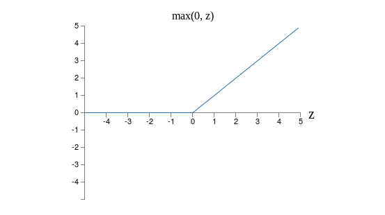
Obviously such neurons are quite different from both sigmoid and tanh neurons. However, like the sigmoid and tanh neurons, rectified linear units can be used to compute any function, and they can be trained using ideas such as backpropagation and stochastic gradient descent.

When should you use rectified linear units instead of sigmoid or tanh neurons? Some recent work on image recognition*

*See, for example, What is the Best Multi-Stage Architecture for Object Recognition?, by Kevin Jarrett, Koray Kavukcuoglu, Marc’Aurelio Ranzato and Yann LeCun (2009), Deep Sparse Rectiﬁer Neural Networks, by Xavier Glorot, Antoine Bordes, and Yoshua Bengio (2011), and ImageNet Classification with Deep Convolutional Neural Networks, by Alex Krizhevsky, Ilya Sutskever, and Geoffrey Hinton (2012). Note that these papers fill in important details about how to set up the output layer, cost function, and regularization in networks using rectified linear units. I’ve glossed over all these details in this brief account. The papers also discuss in more detail the benefits and drawbacks of using rectified linear units. Another informative paper is Rectified Linear Units Improve Restricted Boltzmann Machines, by Vinod Nair and Geoffrey Hinton (2010), which demonstrates the benefits of using rectified linear units in a somewhat different approach to neural networks.

has found considerable benefit in using rectified linear units through much of the network. However, as with tanh neurons, we do not yet have a really deep understanding of when, exactly, rectified linear units are preferable, nor why. To give you the flavor of some of the issues, recall that sigmoid neurons stop learning when they saturate, i.e., when their output is near either $0$ $0$ or $1$ $1$ . As we’ve seen repeatedly in this chapter, the problem is that $\sigma'$ $σ^{'}$ terms reduce the gradient, and that slows down learning. Tanh neurons suffer from a similar problem when they saturate. By contrast, increasing the weighted input to a rectified linear unit will never cause it to saturate, and so there is no corresponding learning slowdown. On the other hand, when the weighted input to a rectified linear unit is negative, the gradient vanishes, and so the neuron stops learning entirely. These are just two of the many issues that make it non-trivial to understand when and why rectified linear units perform better than sigmoid or tanh neurons.

I’ve painted a picture of uncertainty here, stressing that we do not yet have a solid theory of how activation functions should be chosen. Indeed, the problem is harder even than I have described, for there are infinitely many possible activation functions. Which is the best for any given problem? Which will result in a network which learns fastest? Which will give the highest test accuracies? I am surprised how little really deep and systematic investigation has been done of these questions. Ideally, we’d have a theory which tells us, in detail, how to choose (and perhaps modify-on-the-fly) our activation functions. On the other hand, we shouldn’t let the lack of a full theory stop us! We have powerful tools already at hand, and can make a lot of progress with those tools. Through the remainder of this book I’ll continue to use sigmoid neurons as our go-to neuron, since they’re powerful and provide concrete illustrations of the core ideas about neural nets. But keep in the back of your mind that these same ideas can be applied to other types of neuron, and that there are sometimes advantages in doing so.

───

期許未來者乎？？！！

Artificial neuron

An artificial neuron is a mathematical function conceived as a model of biological neurons. Artificial neurons are the constitutive units in an artificial neural network. Depending on the specific model used they may be called a semi-linear unit, Nv neuron, binary neuron, linear threshold function, or McCulloch–Pitts (MCP) neuron. The artificial neuron receives one or more inputs (representing dendrites) and sums them to produce an output (representing a neuron’s axon). Usually the sums of each node are weighted, and the sum is passed through a non-linear function known as an activation function or transfer function. The transfer functions usually have a sigmoid shape, but they may also take the form of other non-linear functions, piecewise linear functions, or step functions. They are also often monotonically increasing, continuous, differentiable and bounded. The thresholding function is inspired to build logic gates referred to as threshold logic; with a renewed interest to build logic circuit resumbling brain processing. For example, new devices such as memristors have been extensively used to develop such logic in the recent times.^[1]

The artificial neuron transfer function should not be confused with a linear system’s transfer function.

……

Basic structure

For a given artificial neuron, let there be m + 1 inputs with signals x₀ through x_m and weights w₀ through w_m. Usually, the x₀ input is assigned the value +1, which makes it a bias input with w_k0 = b_k. This leaves only m actual inputs to the neuron: from x₁ to x_m.

The output of the kth neuron is:

y_{k}=\varphi \left(\sum _{{j=0}}^{m}w_{{kj}}x_{j}\right)

Where $\varphi$ (phi) is the transfer function.

The output is analogous to the axon of a biological neuron, and its value propagates to the input of the next layer, through a synapse. It may also exit the system, possibly as part of an output vector.

It has no learning process as such. Its transfer function weights are calculated and threshold value are predetermined.

Comparison to biological neurons

Artificial neurons are designed to mimic aspects of their biological counterparts.

Dendrites – In a biological neuron, the dendrites act as the input vector. These dendrites allow the cell to receive signals from a large (>1000) number of neighboring neurons. As in the above mathematical treatment, each dendrite is able to perform “multiplication” by that dendrite’s “weight value.” The multiplication is accomplished by increasing or decreasing the ratio of synaptic neurotransmitters to signal chemicals introduced into the dendrite in response to the synaptic neurotransmitter. A negative multiplication effect can be achieved by transmitting signal inhibitors (i.e. oppositely charged ions) along the dendrite in response to the reception of synaptic neurotransmitters.
Soma – In a biological neuron, the soma acts as the summation function, seen in the above mathematical description. As positive and negative signals (exciting and inhibiting, respectively) arrive in the soma from the dendrites, the positive and negative ions are effectively added in summation, by simple virtue of being mixed together in the solution inside the cell’s body.
Axon – The axon gets its signal from the summation behavior which occurs inside the soma. The opening to the axon essentially samples the electrical potential of the solution inside the soma. Once the soma reaches a certain potential, the axon will transmit an all-in signal pulse down its length. In this regard, the axon behaves as the ability for us to connect our artificial neuron to other artificial neurons.

Unlike most artificial neurons, however, biological neurons fire in discrete pulses. Each time the electrical potential inside the soma reaches a certain threshold, a pulse is transmitted down the axon. This pulsing can be translated into continuous values. The rate (activations per second, etc.) at which an axon fires converts directly into the rate at which neighboring cells get signal ions introduced into them. The faster a biological neuron fires, the faster nearby neurons accumulate electrical potential (or lose electrical potential, depending on the “weighting” of the dendrite that connects to the neuron that fired). It is this conversion that allows computer scientists and mathematicians to simulate biological neural networks using artificial neurons which can output distinct values (often from −1 to 1).

───

日	一	二	三	四	五	六
« 5 月				7 月 »
			1	2	3	4
5	6	7	8	9	10	11
12	13	14	15	16	17	18
19	20	21	22	23	24	25
26	27	28	29	30

FreeSandal

每日彙整: 2016-06-24

W!o+ 的《小伶鼬工坊演義》︰神經網絡【百家言】四