是否可能『無限邊界』只包圍『有限面積』??難道真的『重物』跑得比『輕物』較快!!人因懷疑而論辯,因無法實驗而思想︰
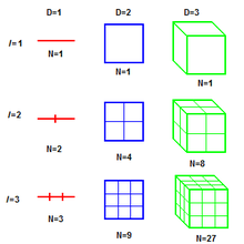
人們『直覺』上都知道,『線』是一維的、『面』是二維的以及『體』是三維的,也許同意『點』是零維的。但是要怎麽定義『維度』 呢?假使設想用一根有刻度的  尺,量一條線段,得到
 ── 單位刻度 ──,如果有另一根
  的尺,它的單位刻度
  是 尺的
是 尺的  倍,也就是說
  ,那用這 之尺來量該線段將會得到
  。同樣的如果 尺量一個正方形得到數值
  ,那用 之尺來量就會得到數值
  ,這樣那
,這樣那 兩尺的度量之數值比
  。
。
於是德國數學家費利克斯‧豪斯多夫 Felix Hausdorff 是這樣子定義『維度』 的︰
的︰

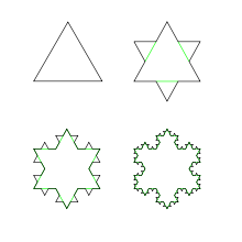
,使它也能適用於『分形』的『分維』。
在科赫雪花的建構過程中,從最初  的 △,到第
  步時︰
步時︰
總邊數︰ 
單一邊長︰ 
總周長︰
圍繞面積︰
因此科赫雪花的分維是

,它所圍繞的極限面積  ,那時的總周長
  。
。
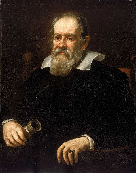

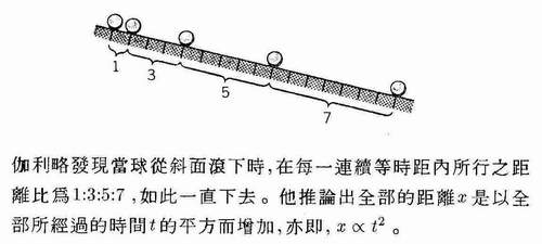

人類天性中的直覺是認識事物、判斷是非和分辨真假非常重要的能力,但是它通常是『素樸的』,所以『概念的分析』也往往是一件『必要的』事。雖然面對『錯綜複雜』的現象,未經粹煉的『思想』容易誤入歧途,但是『直覺理解』的事物,常常流於『想當然耳』之過失。伽利略老年著作了一本『Discorsi e dimostrazioni matematiche』Mathematical Discourses and Demonstrations,據說是『思想實驗』的起始處︰
……
Salviati︰ If then we take two bodies whose natural speeds are different, it is clear that on uniting the two, the more rapid one will be partly retarded by the slower, and the slower will be somewhat hastened by the swifter. Do you not agree with me in this opinion?
Simplicio.︰You are unquestionably right.
Salviati.︰But if this is true, and if a large stone moves with a speed of, say, eight while a smaller moves with a speed of four, then when they are united, the system will move with a speed less than eight; but the two stones when tied together make a stone larger than that which before moved with a speed of eight. Hence the heavier body moves with less speed than the lighter; an effect which is contrary to your supposition. Thus you see how, from your assumption that the heavier body moves more rapidly than ‘ the lighter one, I infer that the heavier body moves more slowly.
……
這段對話用著想像分析、邏輯推導、討論演示著亞里斯多德的『重的東西動得快』的錯誤。概略的說,如果□與○二物重量不同,往同一個方向運動,□也跑得比較 快,設想用一條繩索將這兩者連在一起,那快的應該會被拖慢,而慢的將會被拉快的吧。假使這是件事實,這樣『□+○』整體來看不是更重的東西嗎?難道它不與 『重的東西動得快』矛盾的嗎??
古希臘哲學家埃利亞的芝諾 Ζήνων 宣稱︰即使是參與了特洛伊戰爭古希臘神話中的阿基里斯 Achilles ── 希臘第一勇士 ── 也追不上領先一步之烏龜,因為
動得再慢的物體也不可能被動得更快的物體追上。因為追逐者總得先抵達被逐者上個出發點,然而被逐者此刻早已經前往下個所在點。於是被逐者永遠在追逐者之前一步。
『運動』的概念即使能直覺掌握,卻從來都不是簡單的,就像所有瞬刻都可以說它是『靜止』的『箭矢』,又為什麼不能歸結出『動矢不動』的結論的呢??
─── 摘自《思想實驗!!》
如是者自然喜讀 Michael Nielsen 先生一氣呵成之大哉論也︰
What’s causing the vanishing gradient problem? Unstable gradients in deep neural nets
To get insight into why the vanishing gradient problem occurs, let’s consider the simplest deep neural network: one with just a single neuron in each layer. Here’s a network with three hidden layers:

 are the weights,
  are the biases, and
  is some cost function. Just to remind you how this works, the output
  from the
  th neuron is
  , where
  is the usual sigmoid activation function, and
  is the weighted input to the neuron. I’ve drawn the cost at the end to emphasize that the cost is a function of the network’s output,
  : if the actual output from the network is close to the desired output, then the cost will be low, while if it’s far away, the cost will be high.
We’re going to study the gradient  associated to the first hidden neuron. We’ll figure out an expression for , and by studying that expression we’ll understand why the vanishing gradient problem occurs.
I’ll start by simply showing you the expression for . It looks forbidding, but it’s actually got a simple structure, which I’ll describe in a moment. Here’s the expression (ignore the network, for now, and note that  is just the derivative of the function):

 term in the product for each neuron in the network; a weight
  term for each weight in the network; and a final
  term, corresponding to the cost function at the end. Notice that I’ve placed each term in the expression above the corresponding part of the network. So the network itself is a mnemonic for the expression.
You’re welcome to take this expression for granted, and skip to the discussion of how it relates to the vanishing gradient problem. There’s no harm in doing this, since the expression is a special case of our earlier discussion of backpropagation. But there’s also a simple explanation of why the expression is true, and so it’s fun (and perhaps enlightening) to take a look at that explanation.
Imagine we make a small change  in the bias
  . That will set off a cascading series of changes in the rest of the network. First, it causes a change
  in the output from the first hidden neuron. That, in turn, will cause a change
  in the weighted input to the second hidden neuron. Then a change
  in the output from the second hidden neuron. And so on, all the way through to a change
  in the cost at the output. We have

This suggests that we can figure out an expression for the gradient by carefully tracking the effect of each step in this cascade.
To do this, let’s think about how causes the output  from the first hidden neuron to change. We have
  , so
, so


That  term should look familiar: it’s the first term in our claimed expression for the gradient . Intuitively, this term converts a change in the bias into a change in the output activation. That change in turn causes a change in the weighted input
  to the second hidden neuron:


Combining our expressions for and , we see how the change in the bias propagates along the network to affect  :
:

Again, that should look familiar: we’ve now got the first two terms in our claimed expression for the gradient .
We can keep going in this fashion, tracking the way changes propagate through the rest of the network. At each neuron we pick up a term, and through each weight we pick up a term. The end result is an expression relating the final change in cost to the initial change in the bias:

Dividing by we do indeed get the desired expression for the gradient:

Why the vanishing gradient problem occurs: To understand why the vanishing gradient problem occurs, let’s explicitly write out the entire expression for the gradient:

Excepting the very last term, this expression is a product of terms of the form  . To understand how each of those terms behave, let’s look at a plot of the function :
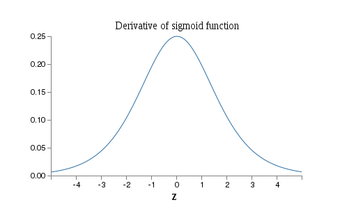
The derivative reaches a maximum at  . Now, if we use our standard approach to initializing the weights in the network, then we’ll choose the weights using a Gaussian with mean
  and standard deviation
  . So the weights will usually satisfy
  . Putting these observations together, we see that the terms will usually satisfy
  . And when we take a product of many such terms, the product will tend to exponentially decrease: the more terms, the smaller the product will be. This is starting to smell like a possible explanation for the vanishing gradient problem.
To make this all a bit more explicit, let’s compare the expression for to an expression for the gradient with respect to a later bias, say  . Of course, we haven’t explicitly worked out an expression for , but it follows the same pattern described above for . Here’s the comparison of the two expressions:
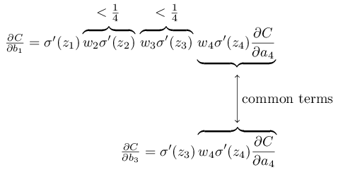 includes two extra terms each of the form . As we’ve seen, such terms are typically less than
  in magnitude. And so the gradient will usually be a factor of
  (or more) smaller than . This is the essential origin of the vanishing gradient problem.
Of course, this is an informal argument, not a rigorous proof that the vanishing gradient problem will occur. There are several possible escape clauses. In particular, we might wonder whether the weights could grow during training. If they do, it’s possible the terms in the product will no longer satisfy . Indeed, if the terms get large enough – greater than – then we will no longer have a vanishing gradient problem. Instead, the gradient will actually grow exponentially as we move backward through the layers. Instead of a vanishing gradient problem, we’ll have an exploding gradient problem.
The exploding gradient problem: Let’s look at an explicit example where exploding gradients occur. The example is somewhat contrived: I’m going to fix parameters in the network in just the right way to ensure we get an exploding gradient. But even though the example is contrived, it has the virtue of firmly establishing that exploding gradients aren’t merely a hypothetical possibility, they really can happen.
There are two steps to getting an exploding gradient. First, we choose all the weights in the network to be large, say  . Second, we’ll choose the biases so that the terms are not too small. That’s actually pretty easy to do: all we need do is choose the biases to ensure that the weighted input to each neuron is
  (and so
  . So, for instance, we want
  . We can achieve this by setting
  . We can use the same idea to select the other biases. When we do this, we see that all the terms are equal to
  . With these choices we get an exploding gradient.
The unstable gradient problem: The fundamental problem here isn’t so much the vanishing gradient problem or the exploding gradient problem. It’s that the gradient in early layers is the product of terms from all the later layers. When there are many layers, that’s an intrinsically unstable situation. The only way all layers can learn at close to the same speed is if all those products of terms come close to balancing out. Without some mechanism or underlying reason for that balancing to occur, it’s highly unlikely to happen simply by chance. In short, the real problem here is that neural networks suffer from an unstable gradient problem. As a result, if we use standard gradient-based learning techniques, different layers in the network will tend to learn at wildly different speeds.
The prevalence of the vanishing gradient problem: We’ve seen that the gradient can either vanish or explode in the early layers of a deep network. In fact, when using sigmoid neurons the gradient will usually vanish. To see why, consider again the expression  . To avoid the vanishing gradient problem we need
  . You might think this could happen easily if
  is very large. However, it’s more difficult than it looks. The reason is that the
  term also depends on :
  , where a is the input activation. So when we make w large, we need to be careful that we’re not simultaneously making
  small. That turns out to be a considerable constraint. The reason is that when we make large we tend to make
  very large. Looking at the graph of you can see that this puts us off in the “wings” of the function, where it takes very small values. The only way to avoid this is if the input activation falls within a fairly narrow range of values (this qualitative explanation is made quantitative in the first problem below). Sometimes that will chance to happen. More often, though, it does not happen. And so in the generic case we have vanishing gradients.
Unstable gradients in more complex networks
We’ve been studying toy networks, with just one neuron in each hidden layer. What about more complex deep networks, with many neurons in each hidden layer?
 th layer of an
  layer network is given by:

Here,  is a diagonal matrix whose entries are the values for the weighted inputs to the lth layer. The
  are the weight matrices for the different layers. And
  is the vector of partial derivatives of with respect to the output activations.
This is a much more complicated expression than in the single-neuron case. Still, if you look closely, the essential form is very similar, with lots of pairs of the form  . What’s more, the matrices
  have small entries on the diagonal, none larger than
  . Provided the weight matrices wj aren’t too large, each additional term
  tends to make the gradient vector smaller, leading to a vanishing gradient. More generally, the large number of terms in the product tends to lead to an unstable gradient, just as in our earlier example. In practice, empirically it is typically found in sigmoid networks that gradients vanish exponentially quickly in earlier layers. As a result, learning slows down in those layers. This slowdown isn’t merely an accident or an inconvenience: it’s a fundamental consequence of the approach we’re taking to learning.