這段文字是本章重點， Michael Nielsen 先生大筆一揮之作。其中的重要性不在於說故事，也不在於談『簡單』與『複雜』到底是誰對誰錯！屬於『信念』的歸『信念』、應該『實證』的得『實證』、有所『懷疑』的當『懷疑』！！如是懷著『科學之心』浸蘊、累積『經驗』久了或能『真知』乎？？

Why does regularization help reduce overfitting?

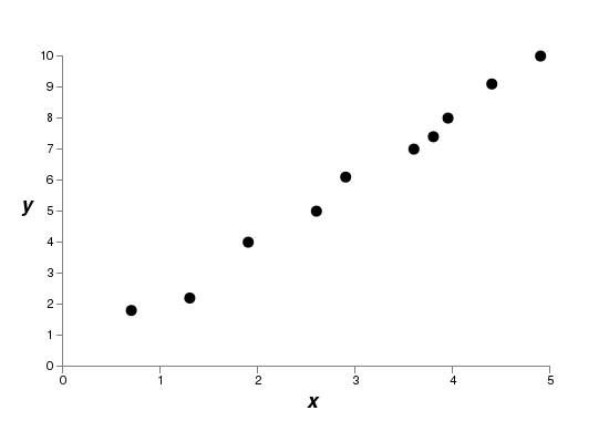
We’ve seen empirically that regularization helps reduce overfitting. That’s encouraging but, unfortunately, it’s not obvious why regularization helps! A standard story people tell to explain what’s going on is along the following lines: smaller weights are, in some sense, lower complexity, and so provide a simpler and more powerful explanation for the data, and should thus be preferred. That’s a pretty terse story, though, and contains several elements that perhaps seem dubious or mystifying. Let’s unpack the story and examine it critically. To do that, let’s suppose we have a simple data set for which we wish to build a model:

Implicitly, we’re studying some real-world phenomenon here, with and representing real-world data. Our goal is to build a model which lets us predict as a function of . We could try using neural networks to build such a model, but I’m going to do something even simpler: I’ll try to model y as a polynomial in . I’m doing this instead of using neural nets because using polynomials will make things particularly transparent. Once we’ve understood the polynomial case, we’ll translate to neural networks. Now, there are ten points in the graph above, which means we can find a unique th-order polynomial which fits the data exactly. Here’s the graph of that polynomial*

*I won’t show the coefficients explicitly, although they are easy to find using a routine such as Numpy’s polyfit. You can view the exact form of the polynomial in the source code for the graph if you’re curious. It’s the function p(x) defined starting on line 14 of the program which produces the graph.:

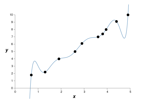
That provides an exact fit. But we can also get a good fit using the linear model :

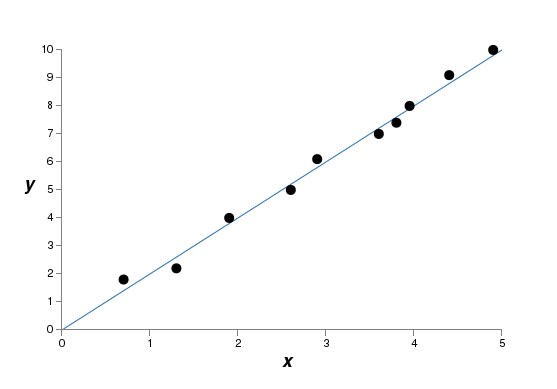
Which of these is the better model? Which is more likely to be true? And which model is more likely to generalize well to other examples of the same underlying real-world phenomenon?

These are difficult questions. In fact, we can’t determine with certainty the answer to any of the above questions, without much more information about the underlying real-world phenomenon. But let’s consider two possibilities: (1) the 9th order polynomial is, in fact, the model which truly describes the real-world phenomenon, and the model will therefore generalize perfectly; (2) the correct model is , but there’s a little additional noise due to, say, measurement error, and that’s why the model isn’t an exact fit.

It’s not a priori possible to say which of these two possibilities is correct. (Or, indeed, if some third possibility holds). Logically, either could be true. And it’s not a trivial difference. It’s true that on the data provided there’s only a small difference between the two models. But suppose we want to predict the value of corresponding to some large value of , much larger than any shown on the graph above. If we try to do that there will be a dramatic difference between the predictions of the two models, as the th order polynomial model comes to be dominated by the term, while the linear model remains, well, linear.

One point of view is to say that in science we should go with the simpler explanation, unless compelled not to. When we find a simple model that seems to explain many data points we are tempted to shout “Eureka!” After all, it seems unlikely that a simple explanation should occur merely by coincidence. Rather, we suspect that the model must be expressing some underlying truth about the phenomenon. In the case at hand, the model seems much simpler than . It would be surprising if that simplicity had occurred by chance, and so we suspect that expresses some underlying truth. In this point of view, the th order model is really just learning the effects of local noise. And so while the 9th order model works perfectly for these particular data points, the model will fail to generalize to other data points, and the noisy linear model will have greater predictive power.

Let’s see what this point of view means for neural networks. Suppose our network mostly has small weights, as will tend to happen in a regularized network. The smallness of the weights means that the behaviour of the network won’t change too much if we change a few random inputs here and there. That makes it difficult for a regularized network to learn the effects of local noise in the data. Think of it as a way of making it so single pieces of evidence don’t matter too much to the output of the network. Instead, a regularized network learns to respond to types of evidence which are seen often across the training set. By contrast, a network with large weights may change its behaviour quite a bit in response to small changes in the input. And so an unregularized network can use large weights to learn a complex model that carries a lot of information about the noise in the training data. In a nutshell, regularized networks are constrained to build relatively simple models based on patterns seen often in the training data, and are resistant to learning peculiarities of the noise in the training data. The hope is that this will force our networks to do real learning about the phenomenon at hand, and to generalize better from what they learn.

With that said, this idea of preferring simpler explanation should make you nervous. People sometimes refer to this idea as “Occam’s Razor“, and will zealously apply it as though it has the status of some general scientific principle. But, of course, it’s not a general scientific principle. There is no a priori logical reason to prefer simple explanations over more complex explanations. Indeed, sometimes the more complex explanation turns out to be correct.

Let me describe two examples where more complex explanations have turned out to be correct.

……

There are three morals to draw from these stories. First, it can be quite a subtle business deciding which of two explanations is truly “simpler”. Second, even if we can make such a judgment, simplicity is a guide that must be used with great caution! Third, the true test of a model is not simplicity, but rather how well it does in predicting new phenomena, in new regimes of behaviour.

With that said, and keeping the need for caution in mind, it’s an empirical fact that regularized neural networks usually generalize better than unregularized networks. And so through the remainder of the book we will make frequent use of regularization. I’ve included the stories above merely to help convey why no-one has yet developed an entirely convincing theoretical explanation for why regularization helps networks generalize. Indeed, researchers continue to write papers where they try different approaches to regularization, compare them to see which works better, and attempt to understand why different approaches work better or worse. And so you can view regularization as something of a kludge. While it often helps, we don’t have an entirely satisfactory systematic understanding of what’s going on, merely incomplete heuristics and rules of thumb.

There’s a deeper set of issues here, issues which go to the heart of science. It’s the question of how we generalize. Regularization may give us a computational magic wand that helps our networks generalize better, but it doesn’t give us a principled understanding of how generalization works, nor of what the best approach is*

*These issues go back to the problem of induction, famously discussed by the Scottish philosopher David Hume in “An Enquiry Concerning Human Understanding” (1748). The problem of induction has been given a modern machine learning form in the no-free lunch theorem (link) of David Wolpert and William Macready (1997)..

……

Let me conclude this section by returning to a detail which I left unexplained earlier: the fact that L2 regularization doesn’t constrain the biases. Of course, it would be easy to modify the regularization procedure to regularize the biases. Empirically, doing this often doesn’t change the results very much, so to some extent it’s merely a convention whether to regularize the biases or not. However, it’s worth noting that having a large bias doesn’t make a neuron sensitive to its inputs in the same way as having large weights. And so we don’t need to worry about large biases enabling our network to learn the noise in our training data. At the same time, allowing large biases gives our networks more flexibility in behaviour – in particular, large biases make it easier for neurons to saturate, which is sometimes desirable. For these reasons we don’t usually include bias terms when regularizing.

───

 

事實上  Michael Nielsen 先生字裡行間透露出過去以來的科學傳統，來自偉大科學家如何進行『科學活動』之『作為典範』。畢竟科學絕非僅止『經驗公式』而已，『理論』之建立，『假說』之設置是為著『理解自然』，故而即使已知許多『現象』是『非線性』的，反倒是先將『線性系統』給研究個徹底。如是方能對比『非線性』系統真實何謂耶？？！！

何謂『線性系統』？ 假使從『系統論』的觀點來看，一個物理系統 ，如果它的『輸入輸出』或者講『刺激響應』滿足

設使 ，，

那 麼

也就是說一個線線系統︰無因就無果、小因得小果，大因得大果 ，眾因所得果為各因之果之總計。

如果一個線性系統還滿足

，這個系統稱作『線性非時變系統』。系統中的『因果關係』是『恆常的』不隨著時間變化，因此『遲延之因』生『遲延之果』 。線性非時變 LTI Linear time-invariant theory 系統論之基本結論是

任何 LTI 系統都可以完全祇用一個單一方程式來表示，稱之為系統的『衝激響應』。系統的輸出可以簡單表示為輸入信號與系統的『衝激響應』的『卷積』Convolution 。

一般物理上所謂的『疊加原理』 Superposition Principle 就是說該系統是一個線性系統。物理上還有一個『局部原理』Principle of Locality 是講︰一個物體的『運動』與『變化』，只會受到它『所在位置』的『周遭影響』。所以此原理排斥『超距作用』，因此『萬有引力』為『廣義相對論』所取代；且電磁學的『馬克士威方程式』取消了『庫倫作用力』。這也就是許多物理學家很在意『量子糾纏』的原因！俗語說『好事不出門， 壞事傳千里』是否是違背了『局部原理』的呢？？

蘇格蘭的哲學家大衛‧休謨 David Hume 經驗論大師，一位徹底的懷疑主義者，反對『因果原理』Causality，認為因果不過是一種『心理感覺』。好比奧地利‧捷克物理學家恩斯特‧馬赫 Ernst Mach  在《Die Mechanik in ihrer Entwicklung, Historisch-kritisch dargestellt》一書中講根本不需要『萬有引力』 之『名』與『因』 ，直接說任何具有質量的兩物間，會有滿足

方程組的就好了；他進一步講牛頓所說的『力』根本是『贅語』，那不過只是物質間的一種『交互作用』interaction 罷了！當真是『緣起性空。萬法歸一，一歸於宗。』的嗎？？

─── 摘自《【Sonic π】聲波之傳播原理︰原理篇《四中》》