光在真空裡與均勻的介質中走直線，直到遭遇不同折射率之界面，或者反射、然而通常多折射，它的軌跡就像『折線』 line chart

 

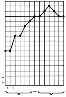
也許這正是『屈光學』名義之由來也。雖說此『折線圖』看來平淡無奇，那要如何描述光之行徑呢？怎樣選取『座標系』才能定位的耶？？光學書本一般將此當成不說自明之理！於是直接展開論述，若干圖例後，難免彷彷彿彿似懂非懂的乎！！

茲舉一圖示為例

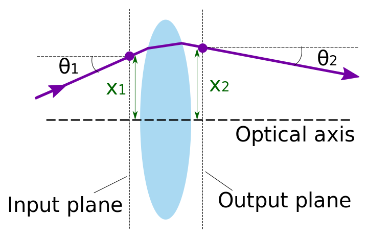
In ray transfer (ABCD) matrix analysis, an optical element (here, a thick lens) gives a transformation between at the input plane and  when the ray arrives at the output plane.

 

，不說那條『折線』？不知『透鏡』厚薄？卻講『輸入面』 input plane 以及『輸出面』 output plane ，圖中強調『光入點』 與『光出點』 之『座標』！宛如『透鏡』在哪無關也！！

假使分解光之『折線圖』的構成，可得『線段』和『轉折點』，那『線段』表示光在『彼介質』中『直行』也，這『轉折點』說明光『此處』發生『反射』或『折射』，而後在『此介質』裡『直行』矣。一個『光學元件』、『光學系統』通常有其物體的『邊界』，如果知道『輸入面』與『輸出面』間 之光線的『行徑關係』，如是這個『光學元件』、『光學系統』的行為就確定了。由於參照自身『邊界面』的原故，因此與其座落『光軸』之何處無關耶？？！！事實上『光軸座標系』乃是一系列『面』與『面』間『相對』位置關係，甚至和『光學元件』、『光學系統』之物體大小不必相涉矣 ！！？？

知此而後知 Justin Peatross 與 Michael Ware 先生們之大哉論也︰

 

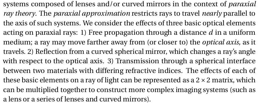
三種基本『光學元素』︰均勻介質裡直線行、球面反射、球面折射的『效應矩陣』足以組成任意複雜之光學成像系統，能夠構造整體『矩陣光學』的了！！！

這裡先列出 sympy Gaussian Optics 之相關文件︰

class sympy.physics.optics.gaussopt.FreeSpace

Ray Transfer Matrix for free space.

Parameters :	distance

Examples

>>> from sympy.physics.optics import FreeSpace
>>> from sympy import symbols
>>> d = symbols('d')
>>> FreeSpace(d)
Matrix([
[1, d],
[0, 1]])

 

class sympy.physics.optics.gaussopt.CurvedRefraction

Ray Transfer Matrix for refraction on curved interface.

Parameters :	R : radius of curvature (positive for concave) n1 : refractive index of one medium n2 : refractive index of other medium

Examples

>>> from sympy.physics.optics import CurvedRefraction
>>> from sympy import symbols
>>> R, n1, n2 = symbols('R n1 n2')
>>> CurvedRefraction(R, n1, n2)
Matrix([
[               1,     0],
[(n1 - n2)/(R*n2), n1/n2]])

 

class sympy.physics.optics.gaussopt.CurvedMirror

Ray Transfer Matrix for reflection from curved surface.

Parameters :	R : radius of curvature (positive for concave)

Examples

>>> from sympy.physics.optics import CurvedMirror
>>> from sympy import symbols
>>> R = symbols('R')
>>> CurvedMirror(R)
Matrix([
[   1, 0],
[-2/R, 1]])

 

再補上一段總綱文字︰

 

循著光踏上自由行乎？？？