學習亦有阻抗乎？俗話說︰

學如逆水行舟，不進則退。

是其阻抗也！然則並非『阻礙之大者』也！？

所以者何？

欲進不得之時，進退維谷之際

不知如之何處之，因而深感難為也？！

故此假借簡單的

RL circuit

A resistor–inductor circuit (RL circuit), or RL filter or RL network, is an electric circuit composed of resistors and inductors driven by a voltage or current source. A first-order RL circuit is composed of one resistor and one inductor and is the simplest type of RL circuit.

A first order RL circuit is one of the simplest analogue infinite impulse response electronic filters. It consists of a resistor and an inductor, either in series driven by a voltage source or in parallel driven by a current source.

Introduction

The fundamental passive linear circuit elements are the resistor (R), capacitor (C) and inductor (L). These circuit elements can be combined to form an electrical circuit in four distinct ways: the RC circuit, the RL circuit, the LC circuit and the RLC circuit with the abbreviations indicating which components are used. These circuits exhibit important types of behaviour that are fundamental to analogue electronics. In particular, they are able to act as passive filters. This article considers the RL circuit in both series and parallel as shown in the diagrams.

In practice, however, capacitors (and RC circuits) are usually preferred to inductors since they can be more easily manufactured and are generally physically smaller, particularly for higher values of components.

Both RC and RL circuits form a single-pole filter. Depending on whether the reactive element (C or L) is in series with the load, or parallel with the load will dictate whether the filter is low-pass or high-pass.

Frequently RL circuits are used for DC power supplies to RF amplifiers, where the inductor is used to pass DC bias current and block the RF getting back into the power supply.

This article relies on knowledge of the complex impedance representation of inductors and on knowledge of the frequency domain representation of signals.

，僅及串聯電路，竟有『如是長篇』說法︰

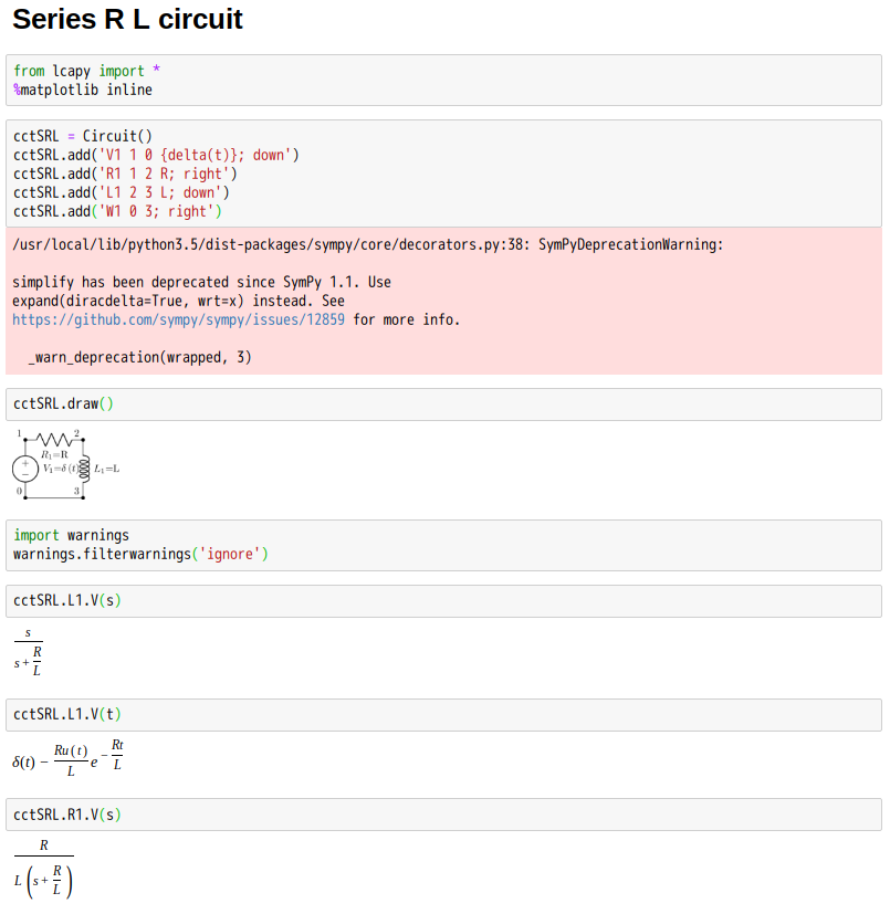
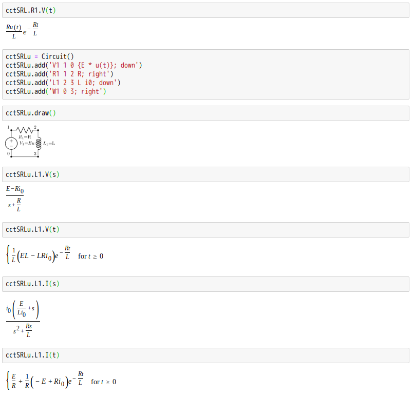
勇猛精進者，當練習

Series circuit

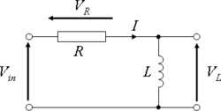
Series RL circuit

By viewing the circuit as a voltage divider, we see that the voltage across the inductor is:

\displaystyle V_{L}(s)={\frac {Ls}{R+Ls}}V_{\mathrm {in} }(s)\,,

and the voltage across the resistor is:

\displaystyle V_{R}(s)={\frac {R}{R+Ls}}V_{\mathrm {in} }(s)\,.

Current

The current in the circuit is the same everywhere since the circuit is in series:

\displaystyle I(s)={\frac {V_{\mathrm {in} }(s)}{R+Ls}}\,.

Transfer functions

The transfer function to the inductor voltage is

\displaystyle H_{L}(s)={\frac {V_{L}(s)}{V_{\mathrm {in} }(s)}}={\frac {Ls}{R+Ls}}=G_{L}e^{j\phi _{L}}\,.

Similarly, the transfer function, to the resistor voltage is

\displaystyle H_{R}(s)={\frac {V_{R}(s)}{V_{\mathrm {in} }(s)}}={\frac {R}{R+Ls}}=G_{R}e^{j\phi _{R}}\,.

The transfer function, to the current, is

\displaystyle H_{I}(s)={\frac {I(s)}{V_{\mathrm {in} }(s)}}={\frac {1}{R+Ls}}\,.

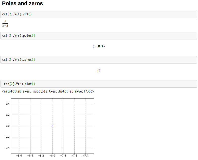
Poles and zeros

The transfer functions have a single pole located at

\displaystyle s=-{\frac {R}{L}}\,.

In addition, the transfer function for the inductor has a zero located at the origin.

Gain and phase angle

The gains across the two components are found by taking the magnitudes of the above expressions:

\displaystyle G_{L}={\big |}H_{L}(\omega ){\big |}=\left|{\frac {V_{L}(\omega )}{V_{\mathrm {in} }(\omega )}}\right|={\frac {\omega L}{\sqrt {R^{2}+\left(\omega L\right)^{2}}}}

and

\displaystyle G_{R}={\big |}H_{R}(\omega ){\big |}=\left|{\frac {V_{R}(\omega )}{V_{\mathrm {in} }(\omega )}}\right|={\frac {R}{\sqrt {R^{2}+\left(\omega L\right)^{2}}}}\,,

and the phase angles are:

\displaystyle \phi _{L}=\angle H_{L}(s)=\tan ^{-1}\left({\frac {R}{\omega L}}\right)

and

\displaystyle \phi _{R}=\angle H_{R}(s)=\tan ^{-1}\left(-{\frac {\omega L}{R}}\right)\,.

Phasor notation

These expressions together may be substituted into the usual expression for the phasor representing the output:

\displaystyle {\begin{aligned}V_{L}&=G_{L}V_{\mathrm {in} }e^{j\phi _{L}}\\V_{R}&=G_{R}V_{\mathrm {in} }e^{j\phi _{R}}\end{aligned}}

Impulse response

The impulse response for each voltage is the inverse Laplace transform of the corresponding transfer function. It represents the response of the circuit to an input voltage consisting of an impulse or Dirac delta function.

The impulse response for the inductor voltage is

\displaystyle h_{L}(t)=\delta (t)-{\frac {R}{L}}e^{-t{\frac {R}{L}}}u(t)=\delta (t)-{\frac {1}{\tau }}e^{-{\frac {t}{\tau }}}u(t)\,,

where $u (t)$ is the Heaviside step function and $τ = L / R$ is the time constant.

Similarly, the impulse response for the resistor voltage is

\displaystyle h_{R}(t)={\frac {R}{L}}e^{-t{\frac {R}{L}}}u(t)={\frac {1}{\tau }}e^{-{\frac {t}{\tau }}}u(t)\,.

Zero-input response

The zero-input response (ZIR), also called the natural response, of an RL circuit describes the behavior of the circuit after it has reached constant voltages and currents and is disconnected from any power source. It is called the zero-input response because it requires no input.

The ZIR of an RL circuit is:

\displaystyle I(t)=I(0)e^{-{\frac {R}{L}}t}=I(0)e^{-{\frac {t}{\tau }}}\,.

Frequency domain considerations

These are frequency domain expressions. Analysis of them will show which frequencies the circuits (or filters) pass and reject. This analysis rests on a consideration of what happens to these gains as the frequency becomes very large and very small.

As $ω \to \infty$ :

\displaystyle G_{L}\to 1\quad {\mbox{and}}\quad G_{R}\to 0\,.

As $ω \to 0$ :

\displaystyle G_{L}\to 0\quad {\mbox{and}}\quad G_{R}\to 1\,.

This shows that, if the output is taken across the inductor, high frequencies are passed and low frequencies are attenuated (rejected). Thus, the circuit behaves as a high-pass filter. If, though, the output is taken across the resistor, high frequencies are rejected and low frequencies are passed. In this configuration, the circuit behaves as a low-pass filter. Compare this with the behaviour of the resistor output in an RC circuit, where the reverse is the case.

The range of frequencies that the filter passes is called its bandwidth. The point at which the filter attenuates the signal to half its unfiltered power is termed its cutoff frequency. This requires that the gain of the circuit be reduced to

\displaystyle G_{L}=G_{R}={\frac {1}{\sqrt {2}}}\,.

Solving the above equation yields

\displaystyle \omega _{\mathrm {c} }={\frac {R}{L}}{\mbox{ rad/s}}\quad {\mbox{or}}\quad f_{\mathrm {c} }={\frac {R}{2\pi L}}{\mbox{ Hz}}\,,

which is the frequency that the filter will attenuate to half its original power.

Clearly, the phases also depend on frequency, although this effect is less interesting generally than the gain variations.

As $ω \to 0$ :

\displaystyle \phi _{L}\to 90^{\circ }={\frac {\pi }{2}}{\mbox{ radians}}\quad {\mbox{and}}\quad \phi _{R}\to 0\,.

As $ω \to \infty$ :

\displaystyle \phi _{L}\to 0\quad {\mbox{and}}\quad \phi _{R}\to -90^{\circ }=-{\frac {\pi }{2}}{\mbox{ radians}}\,.

So at DC (0 Hz), the resistor voltage is in phase with the signal voltage while the inductor voltage leads it by 90°. As frequency increases, the resistor voltage comes to have a 90° lag relative to the signal and the inductor voltage comes to be in-phase with the signal.

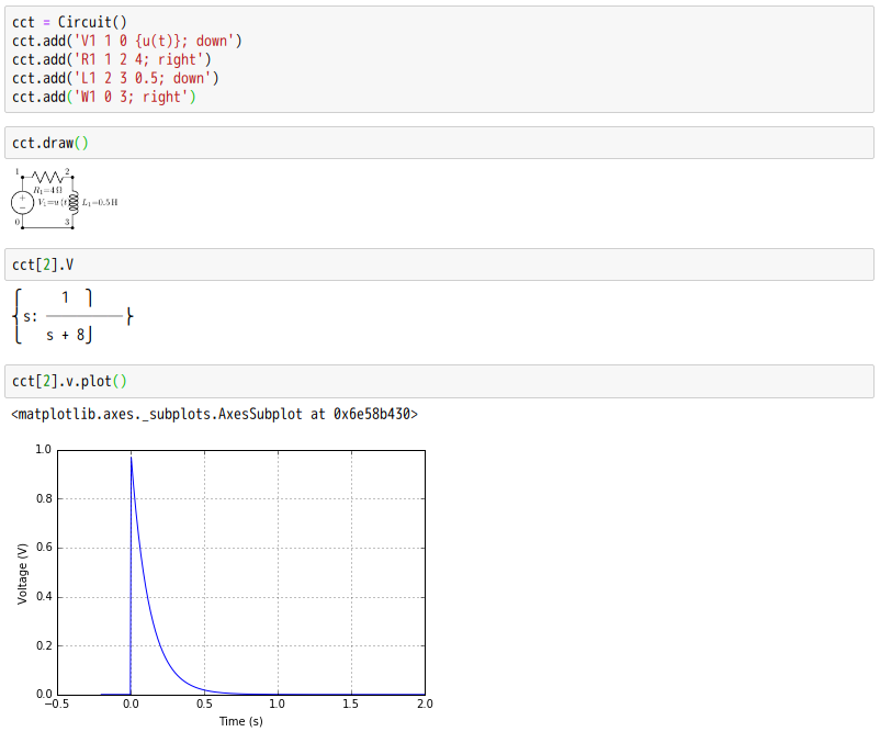
Time domain considerations

The most straightforward way to derive the time domain behaviour is to use the Laplace transforms of the expressions for $V L$ and $V R$ given above. This effectively transforms $jω \to s$ . Assuming a step input (i.e., $V in = 0$ before $t = 0$ and then $V in = V$ afterwards):

\displaystyle {\begin{aligned}V_{\mathrm {in} }(s)&=V\cdot {\frac {1}{s}}\\V_{L}(s)&=V\cdot {\frac {sL}{R+sL}}\cdot {\frac {1}{s}}\\V_{R}(s)&=V\cdot {\frac {R}{R+sL}}\cdot {\frac {1}{s}}\,.\end{aligned}}

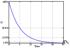
Inductor voltage step-response.

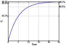
Resistor voltage step-response.

Partial fractions expansions and the inverse Laplace transform yield:

\displaystyle {\begin{aligned}V_{L}(t)&=Ve^{-t{\frac {R}{L}}}\\V_{R}(t)&=V\left(1-e^{-t{\frac {R}{L}}}\right)\,.\end{aligned}}

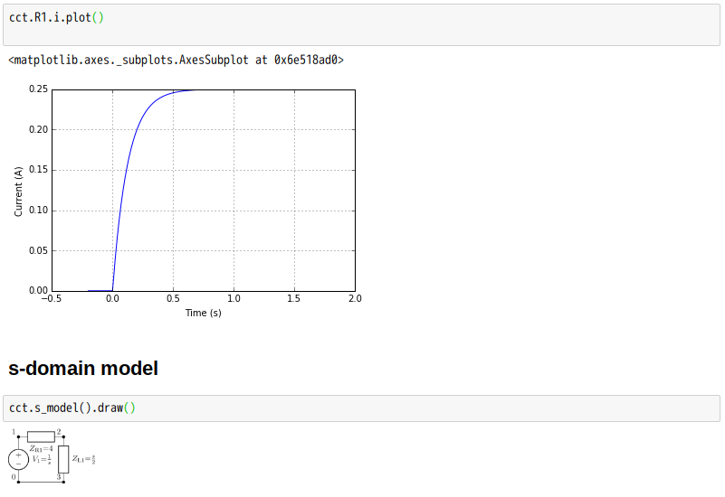
Thus, the voltage across the inductor tends towards 0 as time passes, while the voltage across the resistor tends towards $V$ , as shown in the figures. This is in keeping with the intuitive point that the inductor will only have a voltage across as long as the current in the circuit is changing — as the circuit reaches its steady-state, there is no further current change and ultimately no inductor voltage.

These equations show that a series RL circuit has a time constant, usually denoted $τ = L / R$ being the time it takes the voltage across the component to either fall (across the inductor) or rise (across the resistor) to within $1 / e$ of its final value. That is, $τ$ is the time it takes $V L$ to reach $V (1 / e)$ and $V R$ to reach $V (1 - 1 / e)$ .

The rate of change is a fractional $1 - 1 / e$ per $τ$ . Thus, in going from $t = Nτ$ to $t = (N + 1) τ$ , the voltage will have moved about 63% of the way from its level at $t = Nτ$ toward its final value. So the voltage across the inductor will have dropped to about 37% after $τ$ , and essentially to zero (0.7%) after about $5 τ$ . Kirchhoff’s voltage law implies that the voltage across the resistor will rise at the same rate. When the voltage source is then replaced with a short-circuit, the voltage across the resistor drops exponentially with $t$ from $V$ towards 0. The resistor will be discharged to about 37% after $τ$ , and essentially fully discharged (0.7%) after about $5 τ$ . Note that the current, $I$ , in the circuit behaves as the voltage across the resistor does, via Ohm’s Law.

The delay in the rise or fall time of the circuit is in this case caused by the back-EMF from the inductor which, as the current flowing through it tries to change, prevents the current (and hence the voltage across the resistor) from rising or falling much faster than the time-constant of the circuit. Since all wires have some self-inductance and resistance, all circuits have a time constant. As a result, when the power supply is switched on, the current does not instantaneously reach its steady-state value, $V / R$ . The rise instead takes several time-constants to complete. If this were not the case, and the current were to reach steady-state immediately, extremely strong inductive electric fields would be generated by the sharp change in the magnetic field — this would lead to breakdown of the air in the circuit and electric arcing, probably damaging components (and users).

These results may also be derived by solving the differential equation describing the circuit:

\displaystyle {\begin{aligned}V_{\mathrm {in} }&=IR+L{\frac {dI}{dt}}\\V_{R}&=V_{\mathrm {in} }-V_{L}\,.\end{aligned}}

The first equation is solved by using an integrating factor and yields the current which must be differentiated to give $V L$ ; the second equation is straightforward. The solutions are exactly the same as those obtained via Laplace transforms.