一篇寫得很好的教育論文

Wye-Delta and Delta-Wye Transformations: An Instructive Derivation

Article (PDF Available) in IEEE Transactions on Education 25(4):157-159 · November 1982 with 2,091 Reads

DOI: 10.1109/TE.1982.4321575

A simple derivation of both the wye-delta and delta-wye transformations is presented. This derivation stresses the concept of duality, illustrates the formulation and solution of node and loop matrix equations, and explains the role played by the wye-delta and delta-wye transformations in simplifying circuits.

Full-text (PDF)

Available from: Ali Muhammad Rushdi, Jan 05, 2014

兼容並蓄批判中肯，讀來快意︰

理當大力推薦，自應細心賞析！

若僅抄錄語詞權充註解，豈非貽笑大方之家乎？

Mesh analysis

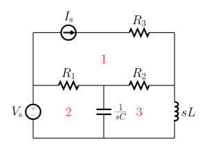
Figure 1: Essential meshes of the planar circuit labeled 1, 2, and 3. R₁, R₂, R₃, 1/sC, and Ls represent the impedance of the resistors, capacitor, and inductor values in the s-domain. V_s and i_s are the values of the voltage source and current source, respectively.

Mesh analysis (or the mesh current method) is a method that is used to solve planar circuits for the currents (and indirectly the voltages) at any place in the electrical circuit. Planar circuits are circuits that can be drawn on a plane surface with no wires crossing each other. A more general technique, called loop analysis (with the corresponding network variables called loop currents) can be applied to any circuit, planar or not. Mesh analysis and loop analysis both make use of Kirchhoff’s voltage law to arrive at a set of equations guaranteed to be solvable if the circuit has a solution.^[1] Mesh analysis is usually easier to use when the circuit is planar, compared to loop analysis.^[2]

Mesh currents and essential meshes

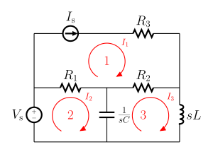
Figure 2: Circuit with mesh currents labeled as i₁, i₂, and i₃. The arrows show the direction of the mesh current.

Mesh analysis works by arbitrarily assigning mesh currents in the essential meshes (also referred to as independent meshes). An essential mesh is a loop in the circuit that does not contain any other loop. Figure 1 labels the essential meshes with one, two, and three.^[3]

A mesh current is a current that loops around the essential mesh and the equations are set solved in terms of them. A mesh current may not correspond to any physically flowing current, but the physical currents are easily found from them.^[2] It is usual practice to have all the mesh currents loop in the same direction. This helps prevent errors when writing out the equations. The convention is to have all the mesh currents looping in a clockwise direction.^[3] Figure 2 shows the same circuit from Figure 1 with the mesh currents labeled.

Solving for mesh currents instead of directly applying Kirchhoff’s current law and Kirchhoff’s voltage law can greatly reduce the amount of calculation required. This is because there are fewer mesh currents than there are physical branch currents. In figure 2 for example, there are six branch currents but only three mesh currents.

Nodal analysis

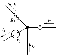
Kirchhoff’s current law is the basis of nodal analysis.

In electric circuits analysis, nodal analysis, node-voltage analysis, or the branch current method is a method of determining the voltage (potential difference) between “nodes” (points where elements or branches connect) in an electrical circuit in terms of the branch currents.

In analyzing a circuit using Kirchhoff’s circuit laws, one can either do nodal analysis using Kirchhoff’s current law (KCL) or mesh analysis using Kirchhoff’s voltage law (KVL). Nodal analysis writes an equation at each electrical node, requiring that the branch currents incident at a node must sum to zero. The branch currents are written in terms of the circuit node voltages. As a consequence, each branch constitutive relation must give current as a function of voltage; an admittance representation. For instance, for a resistor, I_branch = V_branch * G, where G (=1/R) is the admittance (conductance) of the resistor.

Nodal analysis is possible when all the circuit elements’ branch constitutive relations have an admittance representation. Nodal analysis produces a compact set of equations for the network, which can be solved by hand if small, or can be quickly solved using linear algebra by computer. Because of the compact system of equations, many circuit simulation programs (e.g. SPICE) use nodal analysis as a basis. When elements do not have admittance representations, a more general extension of nodal analysis, modified nodal analysis, can be used.

Method

Note all connected wire segments in the circuit. These are the nodes of nodal analysis.
Select one node as the ground reference. The choice does not affect the result and is just a matter of convention. Choosing the node with the most connections can simplify the analysis. For a circuit of N nodes the number of nodal equations is N−1.
Assign a variable for each node whose voltage is unknown. If the voltage is already known, it is not necessary to assign a variable.
For each unknown voltage, form an equation based on Kirchhoff’s current law. Basically, add together all currents leaving from the node and mark the sum equal to zero. Finding the current between two nodes is nothing more than “the node with the higher potential, minus the node with the lower potential, divided by the resistance between the two nodes.”
If there are voltage sources between two unknown voltages, join the two nodes as a supernode. The currents of the two nodes are combined in a single equation, and a new equation for the voltages is formed.
Solve the system of simultaneous equations for each unknown voltage.

就讓我們從電路學對偶現象講起

Duality (electrical circuits)

In electrical engineering, electrical terms are associated into pairs called duals. A dual of a relationship is formed by interchanging voltage and current in an expression. The dual expression thus produced is of the same form, and the reason that the dual is always a valid statement can be traced to the duality of electricity and magnetism.

Here is a partial list of electrical dualities:

voltage – current
parallel – serial (circuits)
resistance – conductance
voltage division – current division
impedance – admittance
capacitance – inductance
reactance – susceptance
short circuit – open circuit
Kirchhoff’s current law – Kirchhoff’s voltage law.
Thévenin’s theorem – Norton’s theorem

History

The use of duality in circuit theory is due to Alexander Russell who published his ideas in 1904.^[1]^[2]

雖然歷史裡『發現』和『發明』之早晚

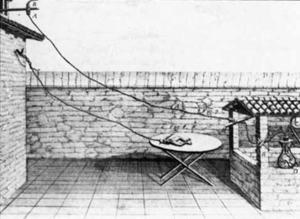
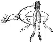
一七八零年義大利醫生、物理學家與哲學家路易吉‧伽伐尼 Luigi Galvani 發現兩種不同的金屬，比方說『銅』和『鋅』連接後，如果一塊兒觸碰青蛙腿的兩處神經，青蛙腿會發生收縮。他將這稱之為『動物電』 animal electricity。傳聞是這麼說的︰

伽伐尼當時正在一張桌子旁，慢慢的給青蛙剝皮。在這張桌子上他曾經用摩擦青蛙皮產生的靜電進行過電學實驗。伽伐尼的助手偶然用一根帶電的金屬解剖刀觸碰了青蛙露在外面的坐骨。這時，伽伐尼和助手看見了火花蹦現，青蛙腿彷彿活著一樣踢了一下。

這使得伽伐尼成為第一個體認到『電』與『生命』有關聯的人。

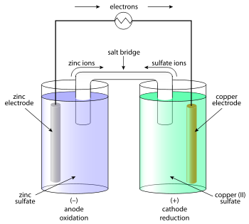
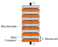
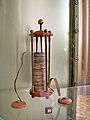
起先義大利物理學家亞歷山德羅‧朱塞佩‧安東尼奧‧阿納斯塔西奧‧伏打 Alessandro Giuseppe Antonio Anastasio Volta 相信『動物電』的說法。而後產生懷疑，再度重複其友伽伐尼的實驗之後，並於一八零零年發明了『伏打電堆』Voltaic pile，是第一個電化學電池，它有『銅』和『鋅』兩個電極，與其間浸有海水的布所構成的單元堆疊而成，今天來看這是一種『電解液』的『氧化還原』化學反應

鋅極 Zinc
$Zn \rightarrow {Zn}^{++} + 2 e^{-}$
銅極 Copper
$2 H^{++} + 2 e^{-} \rightarrow H_2$

，這個電池的單元『電動勢』為 0.76 V『伏特』Volt。一個擁有六個單元的伏打電堆，它的電壓大約是 4.56V。

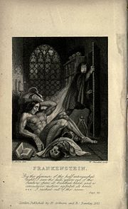
英國著名小說家瑪莉‧雪萊 Mary Shelley 因一八八一年所創作的《弗蘭肯斯坦》 Frankenstein’s monster ── 科學怪人 ── 被譽為科幻小說之母。她曾經提到了伽伐尼的研究報告︰這份研究報告是夏季閱讀書目的一部分，這一書目引發了在瑞士的一次下雨天所進行的一場即席鬼故事大賽，繼而導致了小說《弗蘭肯斯坦》和其中的復活情節的誕生。

因為伏打所得到的這些成果為電池和電學的發展鋪平了道路。於是在一九九九年，伏打電池被正式列名為 IEEE 里程碑！！

─── 摘自《【SONIC Π】電聲學導引《四》》

實非『應用』與『理論』的決定論。

不過在『歐姆定律』 $V = I \cdot R$ 早已朗朗上口的年代， $I = \frac{1}{R} \cdot V$ 又能代表什麼呢？或許只是『電壓產生電流』，計算效應大小罷了！

就像如果有人將太陽

閃焰

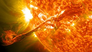
在2012年8月31日爆發的太陽閃焰，曾一直徘徊在太陽的大氣層、日冕，有著長長的日珥/絲狀體噴發至太空中。

閃焰是在太陽的盤面或邊緣觀測到的突發的閃光現象，它會釋放出高達6 × 10²⁵焦耳的巨大能量（大約是太陽每秒鐘釋放總能量的六倍，或相當於160,000,000,000百萬噸TNT，超過舒梅克－李維九號彗星撞木星能量的25,000倍）。它們通常，但並非總是，伴隨著發生日冕大量拋射的事件^[1]。閃焰會從太陽日冕拋射出電子、離子、和原子的雲進入太空。通常，在事件發生後的一兩天，這些雲就可能會到達地球^[2]。這個名詞也適用在發生類似現象的恆星，但通常會使用「恆星閃焰」來稱呼。

閃焰會影響到太陽所有的大氣層（光球、色球和日冕）。當電漿物質被加熱至數千萬K的溫度時，電子、質子和更重的離子都會被加速至接近光速。它們產生電磁頻譜中所有波長的電磁輻射，從無線電波到伽瑪射線，然而絕大部分的能量都在視覺範圍之外，因此絕大碩的閃焰都是肉眼看不見的，必須要用特別的儀器觀測不同的頻率。閃焰發生在圍繞著太陽黑子的活動區，強烈的磁場從那兒穿透光球聯接日冕和太陽內部的磁場。閃焰會突然（時間的尺度在幾分鐘至幾十分鐘）釋放儲藏在日冕中的磁場能量；日冕大量拋射（CME）也可以釋放出相等的能量，但是這兩者之間的關係尚不明確。

閃焰發射的X射線和紫外線輻射會影響地球的電離層，擾亂遠距離的無線電通訊。在分米波長的電波輻射會直接干擾雷達和使用這些波長的儀器和設備的操作。

對太陽閃焰的首度觀測是理查·卡靈頓和理查·霍奇森在1859年獨立完成的^[3]，在黑子群當中看見一個小範圍的明亮區域。觀察望遠鏡或衛星觀測到的恆星光度變化曲線，可以推斷其他恆星是否產生恆星閃焰。

太陽閃焰發的頻率隨著平均11年的活動週期，從太陽位於活躍期的一天數個，到寧靜期的一星期不到一個，有很大的變化（參見太陽週期）。大的閃焰出現的頻率遠低於小的閃焰。

根據NASA的觀測，在2012年7月23日，一個有著巨大和潛在破壞力的太陽超級風暴（閃焰、日冕大量拋射、和太陽電磁脈衝）與地球擦身而過^[4]^[5]。估計在2012年至2022年之間，有12%的機率會發生類似的事件^[4]

成因

閃焰發生時會加速帶電粒子，主要是電子與電漿物質進行交互作用。科學研究表明是磁重聯的現象負責帶電粒子的加速。在太陽，磁重聯可能發在太陽拱圈－一系列密接的磁場線迴圈。這些快速重新連結成迴路的磁場線進入低處，被拱圈其餘為重聯的磁場線纏繞著。這些重聯結時突然釋放的能量是粒子被加速的源頭。未重聯且纏繞在周圍的磁場線和它所包含的物質可能會猛烈的向外擴張，形成日冕大量拋射^[6]。這也解釋了為什麼閃焰的爆發通常都在磁場較為強烈，也比平均活躍的活動區。

雖然，這是一般所認同的閃焰成因，但細節仍不為人所知。尚不清楚磁場的能量如何轉化為粒子的動能，也不知道如何將粒子加速，甚至超越千萬電子伏特的能量。對於被加速粒子的總數，有時似乎總是大於迴圈中粒子數量的不一致性，也尚無法解決。即使在現在，科學家還是無法預測閃焰^{[來源請求]}。

連及

Current source

A current source is an electronic circuit that delivers or absorbs an electric current which is independent of the voltage across it.

A current source is the dual of a voltage source. The term current sink is sometimes used for sources fed from a negative voltage supply. Figure 1 shows the schematic symbol for an ideal current source driving a resistive load. There are two types. An independent current source (or sink) delivers a constant current. A dependent current source delivers a current which is proportional to some other voltage or current in the circuit.

生關聯，也難說全錯的耶？

假設將一個有 $n$ 『端點』的『電路』或『元件』看成『黑箱』，它的『參考於地』之『端點電壓』 $V_i , \ i = 1 \cdots n$ ，最多只能形成 $n-1$ 個『電位差』。

為了方便表述起見，且用 $V_n$ 當作『電壓參考點』，那麼 $I_k, \ k = 1 \cdots n-1$ 就是獨有 $Vk,n = V_k - V_n$ 『電壓源』之時，流入『端點』 $k$ 的『電流』也。

既是『線性系統』，故遵循

$\displaystyle {\begin{bmatrix}I_{1}\\I_{2}\\\vdots \\I_{n-1}\end{bmatrix}} ={\begin{bmatrix}G_{1,1}&G_{1,2}&\cdots &G_{1,{n-1}}\\G_{2,1}&G_{2,2}&\cdots &G_{2,{n-1}}\\\vdots &\vdots &\ddots &\vdots \\G_{{n-1},1}&G_{{n-1},2}&\cdots &G_{{n-1},{n-1}}\end{bmatrix}} \ {\begin{bmatrix}V_{1,n}\\V_{2,n}\\\vdots \\V_{{n-1},n}\end{bmatrix}}$

滿足『疊加原理』呦。

$\displaystyle = {\begin{bmatrix}G_{1,1}&G_{1,2}&\cdots &G_{1,{n-1}}\\G_{2,1}&G_{2,2}&\cdots &G_{2,{n-1}}\\\vdots &\vdots &\ddots &\vdots \\G_{{n-1},1}&G_{{n-1},2}&\cdots &G_{{n-1},{n-1}}\end{bmatrix}} \ \left( {\begin{bmatrix}V_{1,n}\\0\\\vdots \\0\end{bmatrix}} +\left( {\begin{bmatrix} 0\\V_{2,n}\\\vdots \\0\end{bmatrix}} + \cdots + {\begin{bmatrix}0\\0\\\vdots \\V_{{n-1},n}\end{bmatrix}} \right)$

因此『線性獨立』之 wye

$\displaystyle {\begin{bmatrix}I_{a}\\I_{b} \end{bmatrix}} = \frac{1}{Z_1 Z_2 + Z_2 Z_3 + Z_3 Z_1} \ {\begin{bmatrix} Z_2 + Z_3 & -Z_3 \\ -Z_3& Z_1 + Z_3 \end{bmatrix}} \ {\begin{bmatrix} -V_{ca}\\V_{bc} \end{bmatrix}}$

必然『存在』 Y-Δ_transform 哩◎

承上篇︰

$\displaystyle {\begin{bmatrix}I_{a}\\I_{b} \end{bmatrix}} = \frac{-V_{ca}}{Z_1 Z_2 + Z_2 Z_3 + Z_3 Z_1} \ {\begin{bmatrix} Z_2 + Z_3 \\ -Z_3 \end{bmatrix}}$

$\therefore I_c = \frac{- Z_2}{Z_1 Z_2 + Z_2 Z_3 + Z_3 Z_1} (-V_{ca})$

$\displaystyle {\begin{bmatrix}I_{a}\\I_{b} \end{bmatrix}} = \frac{V_{bc}}{Z_1 Z_2 + Z_2 Z_3 + Z_3 Z_1} \ {\begin{bmatrix} - Z_3 \\ Z_1 + Z_3 \end{bmatrix}}$