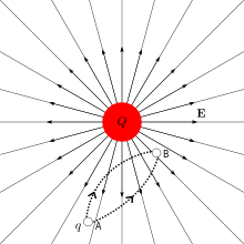
假使一個帶電荷量為 q 的粒子在電場 $\vec{E}$ 中從 A 點移動到 B 點，此電場力所做的『功』 $W_{AB}$ 與電荷量 q 的『比值』，稱之為 AB 兩點間的『電位差』，可用 $V_{AB}=\frac{W_{AB}}{q}$ 定義。『電位差』在『電磁學』裡也可以用電場 $\vec{E}$ 表示為︰
$V_{AB} = V_A - V_B = - \int_{r_0}^{A} \vec{E} \cdot d\vec{l} - \left( - \int_{r_0}^{B} \vec{E} \cdot d\vec{l} \right)$
$= \int_{A}^{r_0} \vec{E} \cdot d\vec{l} + \int_{r_0}^{B} \vec{E} \cdot d\vec{l} = \int_{A}^{B} \vec{E} \cdot d\vec{l}$
。因此所謂的『一伏特』One Volt 的定義就是對『一庫侖』的電荷做了『一焦耳』的功。

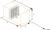
如果我們從『巨觀現象』的角度，來看『德汝德模型』，通常一個『截面均勻』的導體之『電阻』或『電阻率』和導體『長度』成正比，與其『截面積』成反比。這可以用關係式表達為 $R=\rho\frac{\ell}{A}$ ，此處， R 是電阻， $\ell$ 是長度， A 是截面積， $\rho$ 是電阻率。假使根據『歐姆定律』，電壓 V 等於電流 I 乘上電阻： $V = I R$ 。所以，
$V = I \rho\frac{\ell}{A}$ 。由於在均勻導體內，『電場』與『電壓』的關係為
$\vec{E} = \frac{V}{\ell}\hat{z}$ ；
式中， $\hat{z}$ 是電流方向。因此，
$\vec{E}=\rho\frac{I}{A}\hat{z} = \rho \vec{J}$ 。
因為『電導率』是『電阻率』的倒數， $\sigma=1/\rho$ 。於是『電流密度』與『電場』的關係為
$\vec{J}=\sigma\vec{E}$ 。將它與『微觀』推導方程式作比較，就可以得到

$\sigma = \left( \frac{n q^2 \tau}{m} \right)$ 。

因此只要知道導體的『電導率』或者『電阻率』，我們能夠計算『弛豫時間』 $\tau$ 的大小，舉例來說『鈉』在 20 °C時的『電阻率』是 $47.7 \times {10}^{-9}$ 歐姆‧米，於是它的『弛豫時間』是

$\frac{9.109 \times {10}^{-31}} {47.7 \times {10}^{-9} \cdot {\left( 1.602 \times {10}^{-19} \right)}^2 \cdot 2.54 \times {10}^{28}} = 2.93 \times {10}^{-14}$

秒。這說明了我們很難觀測到『暫態』的現象，一般金屬『導體』幾乎是『瞬間』就達到了『穩態』！！

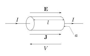
這樣什麼又是『電流』的呢？從『微觀』上來說，如果一條『導線』在『一秒鐘』內，對於任何的『截面』上，通過了相當於『一庫侖』的『電荷量』所指稱之 $6.242 \times {10}^{18}$ 這麼多個『電子』的數量，我們就將此『電流』定義為是『一安培』。由是對於一個『穩定』的『電流』來講，這條導線上流經之『電流』 I 就可以用下式來計算：

$I = {\Delta Q \over \Delta T}$

此處， $\Delta Q$ 是那個時距所通過的『電荷量』， $\Delta T$ 則是它所花費的『時距』。

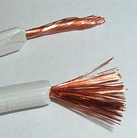
那麼為什麼金屬『導體』它可以傳導這麼大的『電流量』的呢？？這就是因為『金屬』的『電子密度』非常高的原故。假使我們用『銅線』的『美國線規』 AWG American wire gauge 來講，『十四號』線材的『直徑』為一點六二八公釐，即使它祇是一公釐長的銅線，每個銅原子也祇貢獻一個『自由電子』，其中尚且含有 $3.51 \times {10}^{20}$ 個電子，相當於五十六『庫倫』的『電荷量』，無怪乎就算是那麼小的『漂移速度』，依然是可以負載這麼大的『電流』量的啊！！

─── 《【SONIC Π】電聲學補充《三》中》

如果知道『歐姆定律』，明白了『電阻』由來之『微觀解釋』，不知能否設想如何精確測量『電阻』呢？

四端點測量技術

四端測試法

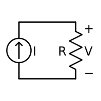
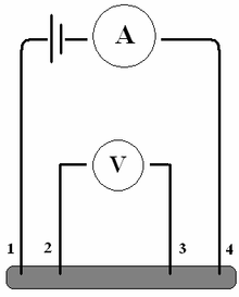
四端點測量技術，又稱為四端測試法，開爾文測量法，是一種電子線路中的阻抗測量法，主要用於電阻阻值的精確測量。根據歐姆定律， $\displaystyle R=V/I\,\!$ ，電阻阻值的測量可通過測量電阻兩端電壓U與流經電阻的電流I來實現。不論是近距離還是遠距離測量阻值，測量結果都會受到導線壓降的影響而造成精確度的損失，遠距離測量時由於導線造成的壓降更大而造成不可忽略的影響。下圖為理想的測量情形，電壓表直接測得電阻兩側電壓，此測量結果未受導線壓降影響。

然而實際測量中受限於某些條件而只能遠距離測量電壓^[1]，此時由於遠距離測量中大電流流經長導線造成了不可忽視的壓降，而對測量電阻阻值造成影響。解決此問題的一個方案就是四端點測量技術。採用下圖方案，遠距離測量時，電壓表便無需被置於被測電阻處，而是由單獨導線引至電流表附近。由於流經此單獨導線的電流值（亦即電壓表電流值）與流經被測電阻的電流值相比，小到近似可以忽略（電壓表內阻極大），因此支路導線未造成足夠影響測量結果的壓降，此時所測電壓與電流表所測電流之比可近似認為是被測電阻阻值。此原理同樣適用於近距離精準測量。

就像『電路學』之『知識』與應用 lcapy 『分析工具』的『方法』

One-port networks
—————–

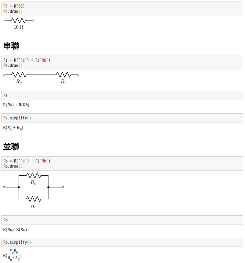
One-port networks can be created by series and parallel combinations
of other one-port networks. The primitive one-port networks are the
following ideal components:

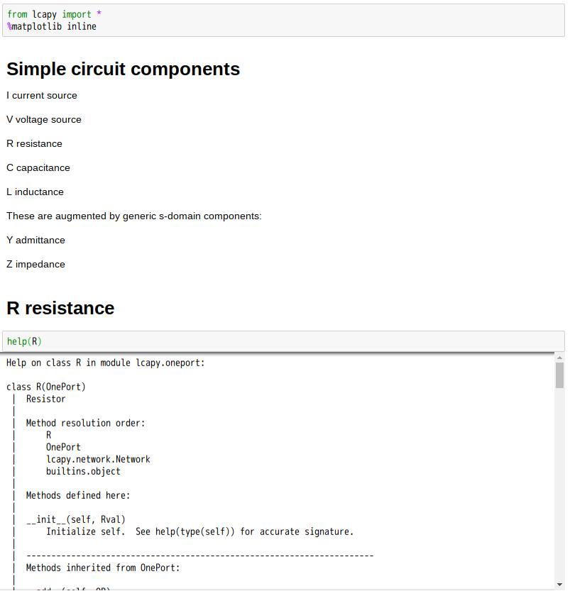
V independent voltage source
I independent current source
R resistor
C capacitor
L inductor

These components are converted to s-domain models and so capacitor and
inductor components can be specified with initial voltage and
currents, respectively, to model transient responses.

The components have the following attributes:

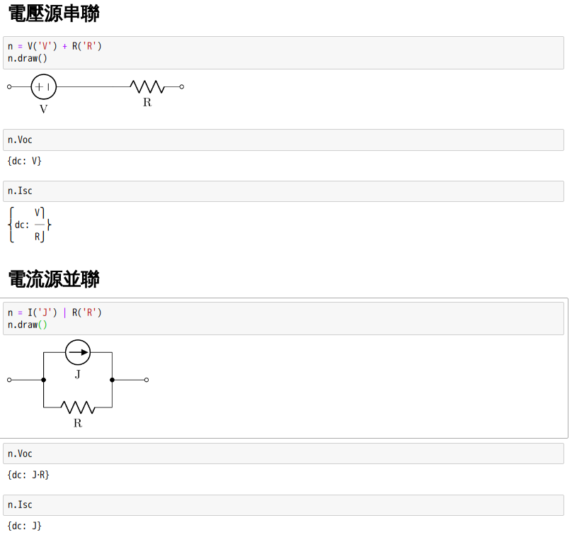
Zoc open-circuit impedance
Ysc short-circuit admittance
Voc open-circuit voltage
Isc short-circuit current

The component values can be specified numerically or symbolically
using strings, for example,

from lcapy import Vdc, R, L, C

>>> R1 = R(‘R_1’)
>>> L1 = L(‘L_1’)
>>> a = Vdc(10) + R1 + L1

Here a is the name of the network formed with a 10 V DC voltage source in
series with R1 and L1.

The s-domain open circuit voltage across the network can be printed with:
>>> a.Voc.s
10/s

The time domain response is given by:
>>> a.Voc.transientresponse()
10*Heaviside(t)

The s-domain short circuit current through the network can be printed with:
>>> a.Isc.s
10/(L_1*s**2 + R_1*s)

The time domain response is given by:
>>> a.Isc.transientresponse()
10*Heaviside(t)/R_1 – 10*exp(-R_1*t/L_1)*Heaviside(t)/R_1
Two-port networks
—————–

One-port networks can be combined to form two-port networks. Methods
are provided to determine transfer responses between the ports.

Here’s an example of creating a voltage divider (L section)

>>> a = LSection(R(‘R_1’), R(‘R_2’))
Limitations
———–

1. Non-linear components cannot be modelled (apart from a linearisation around a bias point).

2. High order systems can go crazy.

3. Some two-ports generate singular matrices.

………

不同呦！

特先告訴讀者，此系列串講未依